Warning: This review is a work in progress
Observational Astronomy
I had decided to follow an Oxford University Summer School (2026) on the subject “Exploring the Cosmos: Technology, Theory, and Discovery”.
One of the recommended reading was “Observational Astronomy” by Geoff Cottrell. It’s from the Oxford University Press, and is subtitled “A Very Short Introduction“.
I have prepared notes on Chapter 1 (The Observable Universe) and 2 (Big Telescopes). So here I am in revision-note-mode for Chapter 3 on…
The Radio Universe
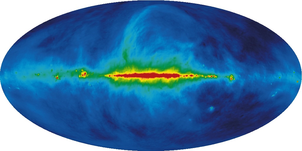
Above we have a full-sky image of the radio brightness of the sky at a frequency of 408 MHz (wavelength ≈ 73 cm), in the metre-wave radio band. It shows the sky in terms of radio continuum emission, dominated by diffuse synchrotron radiation from the Milky Way, produced by relativistic electrons spiralling in the Galactic magnetic field. We see the bright emission along the Galactic plane, where cosmic-ray density and magnetic fields are strongest. The discrete bright structures are supernova remnants and large radio loops, and the fainter, nearly uniform background including unresolved extragalactic radio sources. So it’s a global view of the Milky Way as a radio-emitting galaxy, rather than a star-light image.
The original survey was carried out in the late 1960s–early 1980s using several large single-dish radio telescopes covering both hemispheres, in order to map the entire sky at 408 MHz. This actual image is from 2014 and is a cleaned and digitally improved version of the original Haslam map.
First, check out the following introductory videos:-
History of Radio Astronomy, an accessible and broad historical introduction from the Green Bank Observatory.
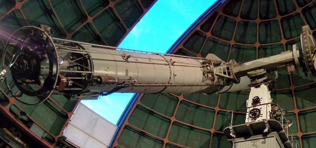
The New Era of Radio Astronomy, probably a better, but equally accessible, technical description, and in particular looking at those telescopes that don’t look like telescopes.
The Revolution in Radio Astronomy with a bit of history, and a particular mention of Australian Square Kilometre Array Pathfinder (ASKAP) and the future Square Kilometre Array (SKA). Includes an extended mention of Fast Radio Bursts.
Beyond the Visible: The Story of the Very Large Array, (overly) simple, but a well packaged description of a well known centimetre-wavelength radio telescope array in New Mexico.
Early days…
Karl Guthe Jansky (1905-1950) was a radio engineer who in April 1933 first announced his discovery of radio waves emanating from the Milky Way in the constellation Sagittarius.
At Bell Telephone Laboratories, Jansky built a directional antenna designed to receive radio waves at a frequency of 20.5 MHz (wavelength about 14.6 meters). It had a diameter of approximately 30 meters and stood 6 meters tall. After recording signals from all directions for several months, Jansky eventually categorised them into three types of static, namely nearby thunderstorms, distant thunderstorms, and a faint static or “hiss” of unknown origin. He spent over a year investigating the source of the third type of static. The location of maximum intensity rose and fell once a day, leading Jansky to surmise initially that he was detecting radiation from the Sun.
After a few months of following the signal, however, the point of maximum static moved away from the position of the Sun. Jansky also determined that the signal repeated on a cycle of 23 hours and 56 minutes. Jansky discussed the puzzling phenomena with his friend the astrophysicist Albert Melvin Skellett, who pointed out that the observed time between the signal peaks was the exact length of a sidereal day, the time it took for “fixed” astronomical objects, such as a star, to pass in front of the antenna every time the Earth rotated. By comparing his observations with optical astronomical maps, Jansky concluded that the radiation was coming from the Milky Way and was strongest (7:10 p.m. on September 16, 1932) in the direction of the centre of the galaxy, in the constellation of Sagittarius.
Jansky announced his discovery at a meeting in Washington D.C. in April 1933, but he found little support from astronomers. Later Jansky noise is named after him, and refers to high frequency static disturbances of cosmic origin, cosmic noise. Also the Jansky is a non-SI unit of spectral flux density, or spectral irradiance, used especially in radio astronomy.
In 1937 Grote Reber, a radio engineer built a radio telescope (a 9-metre parabolic sheet metal dish) in his back yard and conducted the first sky survey in the radio frequencies. Also John D. Kraus started a radio observatory at Ohio State University and wrote a textbook on radio astronomy, long considered a standard by radio astronomers. In 1944 Reber went on to publish the first rough radio map, confounding astronomers because the position of the maximum radio emission was some 30° off the then accepted Galactic centre.
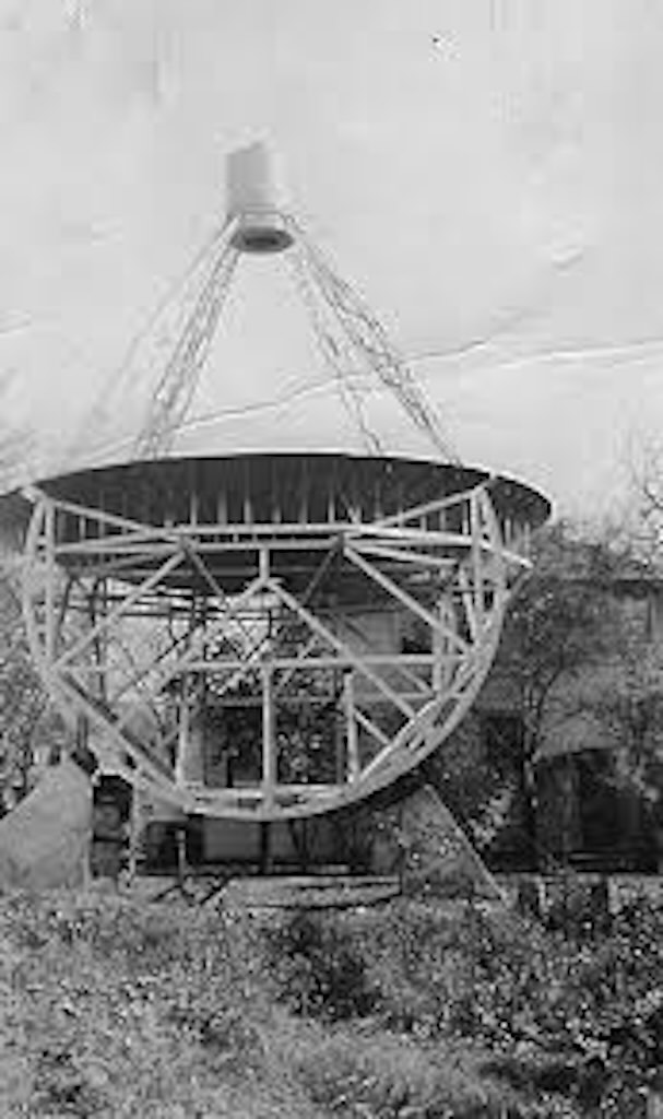
Reber decided he wanted to find out whether the sky contained more radio sources. Since no university or observatory was building radio telescopes, Reber built one himself in his backyard in Wheaton, Illinois, beginning in 1937. It was the first purpose-built radio telescope used for astronomy. And it had what are not the classical elements of a radio telescope, i.e. a 9.5-metre diameter parabolic optical reflector dish mounted so it could be steered across the sky, with a receiver placed at the focus. Reber built and rebuilt his receivers from scratch several times, eventually succeeding at frequencies around 160 MHz. Between 1939 and 1944, working alone, Reber produced the first systematic radio survey of the sky, the first radio maps of the Milky Way, and proof that radio astronomy was a real observational science. But no major observatories followed up his work until after WWII, when radar technology had produced skilled engineers and better receivers.
The spectrum of a star is composed mainly of thermal radiation that produces a continuous spectrum. Thermal radiation is just electromagnetic radiation emitted by the thermal motion of particles in matter. All matter with a temperature greater than absolute zero emits thermal radiation. The emission of energy arises from a combination of electronic, molecular, and lattice oscillations in a material. Kinetic energy is converted to electromagnetism due to charge-acceleration or dipole oscillation. The primary method by which a star (like the Sun) transfers heat is thermal radiation. Cosmic microwave background radiation is another example of thermal radiation.
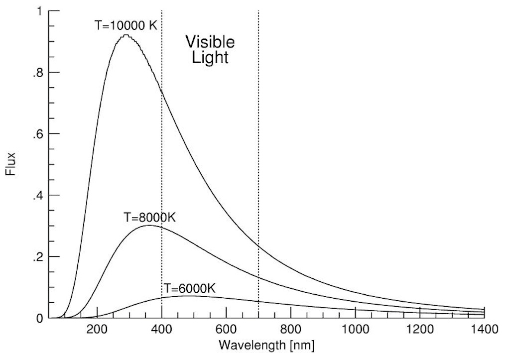
Planck’s law describes the spectrum of blackbody radiation, and relates the radiative flux from a body to its temperature (see above). Wien’s displacement law determines the most likely frequency of the emitted radiation, and the Stefan–Boltzmann law gives the radiant intensity. A star emits light over the entire electromagnetic spectrum, from gamma rays to radio waves. However, stars do not emit the same amount of energy at all wavelengths. The peak emission of their thermal radiation (the continuum peak) comes at a wavelength determined by the star’s surface temperature, and the hotter the star, the bluer the continuum peak. In addition to the continuous spectrum, a star’s spectrum includes a number of dark lines (absorption lines).
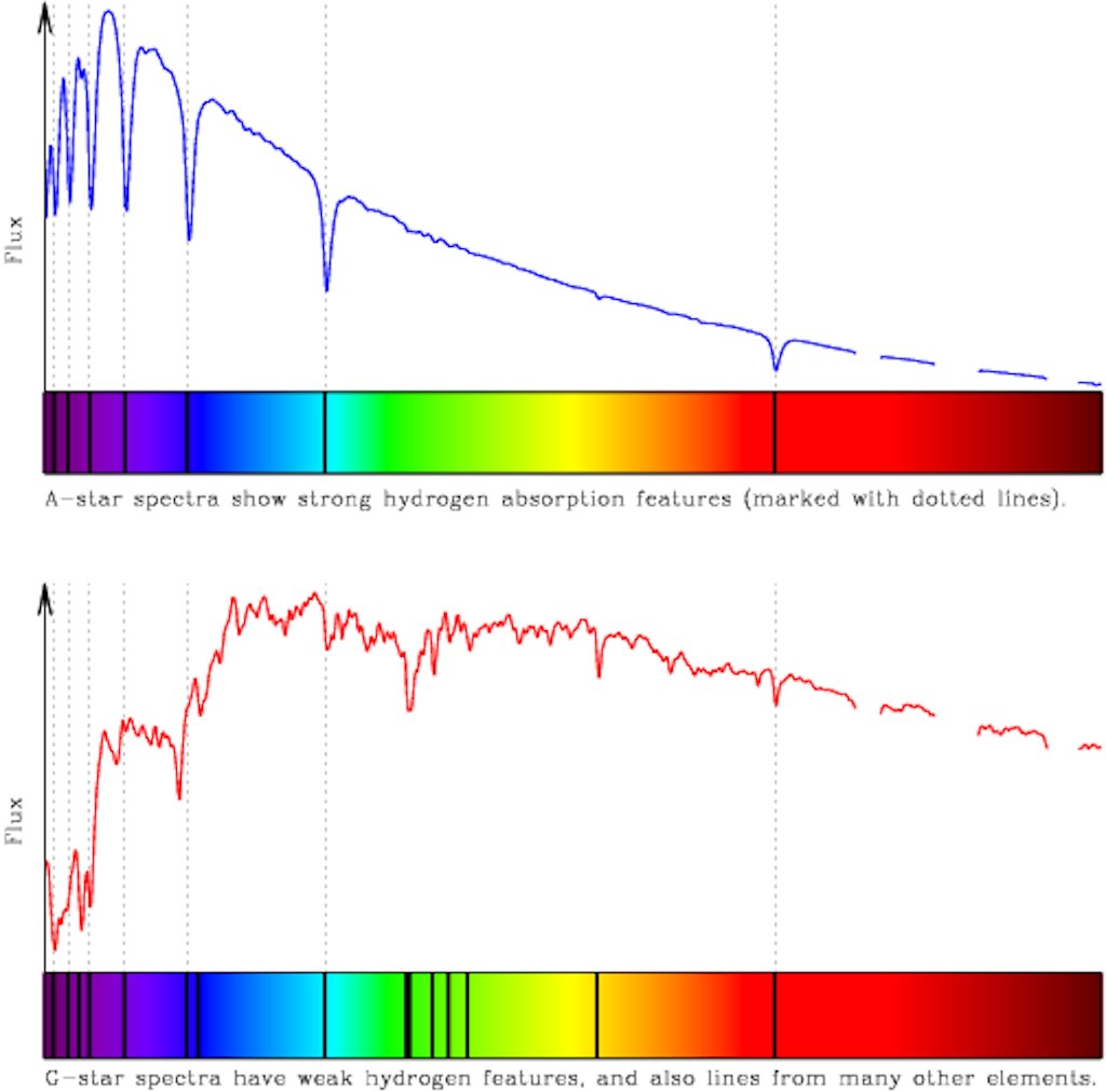
An A-star is a white to bluish-white star much hotter and brighter than the Sun, which is a G-star. Type “A” has the strongest hydrogen absorption lines, and a G-star has weak hydrogen lines.
Absorption lines are produced by atoms whose electrons absorb light at a specific wavelength, causing the electrons to move from a lower energy level to a higher one. This process removes some of the continuum being produced by the star and results in dark features in the spectrum.
In astronomical spectroscopy, the strength, shape, and position of absorption and emission lines, as well as the overall spectral energy distribution of the continuum, reveal many properties of astronomical objects. Stellar classification is the categorisation of stars based on their characteristic electromagnetic spectra. The spectral flux density is used to represent the spectrum of a light-source, such as a star.
However, the radio noise emitted by the Milky Way does not have the same form of thermal spectrum as emitted by stars, nor does it have discrete absorption lines. As mentioned above the centre of the Milky Way was the first radio source to be detected. It contains a number of radio sources, including Sagittarius A, the compact region around the supermassive black hole, Sagittarius A*, as well as the black hole itself. When flaring, the accretion disk around the supermassive black hole lights up, creating detectable in radio waves.
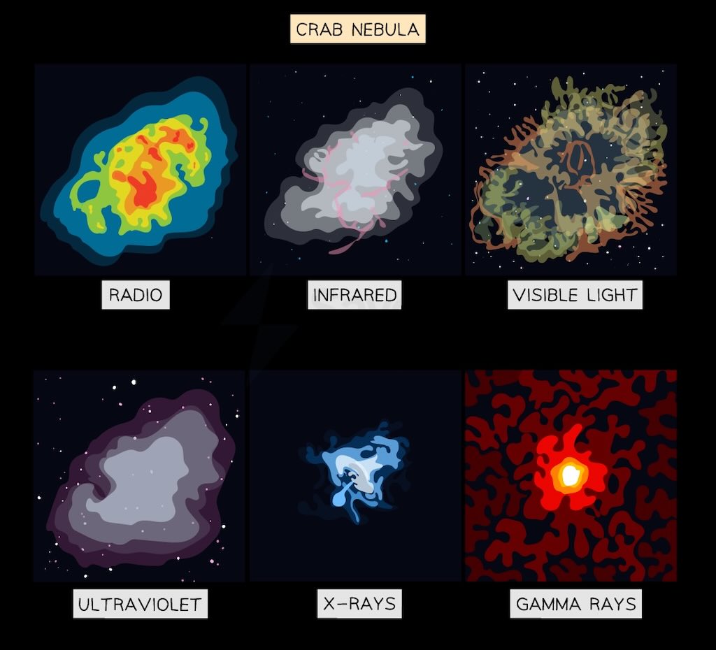
Above we can see the Crab Nebula in different wavelengths.
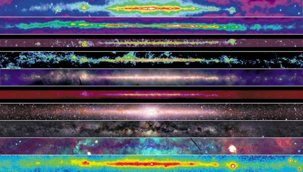
Above we have multiple views of the Milky Way. Starting from the top, we have the radio continuum (408 MHz), next atomic hydrogen, radio continuum (2.5 GHz), molecular hydrogen, infrared, mid-infrared, near infrared, optical, X-ray and finally gamma-ray.
The linear polarisation of the Galactic radio waves was discovered in 1962 and was thought to be the ‘missing link’ in the interpretation of the radio continuum emission. These observations were interpreted as consistent with synchrotron radiation from relativistic electrons in the Galactic magnetic field. Polarisation traced the direction and organisation of magnetic fields across the Galaxy. It pointed to synchrotron radiation produced by relativistic electrons (one form of cosmic rays) moving through a magnetic field. And that the radio waves must pass through ionised gas, where the polarisation angle rotates (Faraday rotation). They deduced this because what they actually observed was a changing polarisation angle at different radio frequencies (so they didn’t need to know the original direction of polarisation).
When radio astronomers first detected strong linear polarisation in cosmic radio sources, they were shocked because most familiar radiation sources were essentially unpolarised. Stars emit mostly thermal light, which is weakly polarised, hot gases the same, so the expectation was that cosmic radio noise should be mostly random in polarisation. But it wasn’t. In fact, solar radio emission showed polarisation as early as 1946, and the Crab Nebula’s radio emission was found to be linearly polarised in the 1950s. So the concept and measurement of radio polarisation in astronomy were already established before 1962. But this exact year is often cited because Ronald N. Bracewell used the Parkes Observatory 64 m radio telescope to confirmed strong linear polarisation in an extragalactic source (Centaurus A), not just within the Milky Way or supernova remnants. So 1962 is quoted because it showed that magnetic fields and synchrotron physics were not just local features but cosmic ones.
Radio astronomers already knew in the 1950s that synchrotron theory existed and that polarisation might be expected, but it could have been treated as a special, or localised, case. The 1962 result established that polarisation was widespread rather than exceptional, and that magnetised relativistic plasmas shape galaxies and the cosmos.
As a reminder, synchrotron radiation is associated with the acceleration that happens to electrons as they spiral around a magnetic field. The force felt by a charged particle in a magnetic field is perpendicular to the direction of the field and to the direction of the particle’s velocity. The net effect of this is to cause the particle to spiral around the direction of the field. Since circular motion represents acceleration (i.e. a change in velocity), the electrons radiate photons of a characteristic energy, corresponding to the radius of the circle. For non-relativistic motion, this is called “cyclotron radiation“.
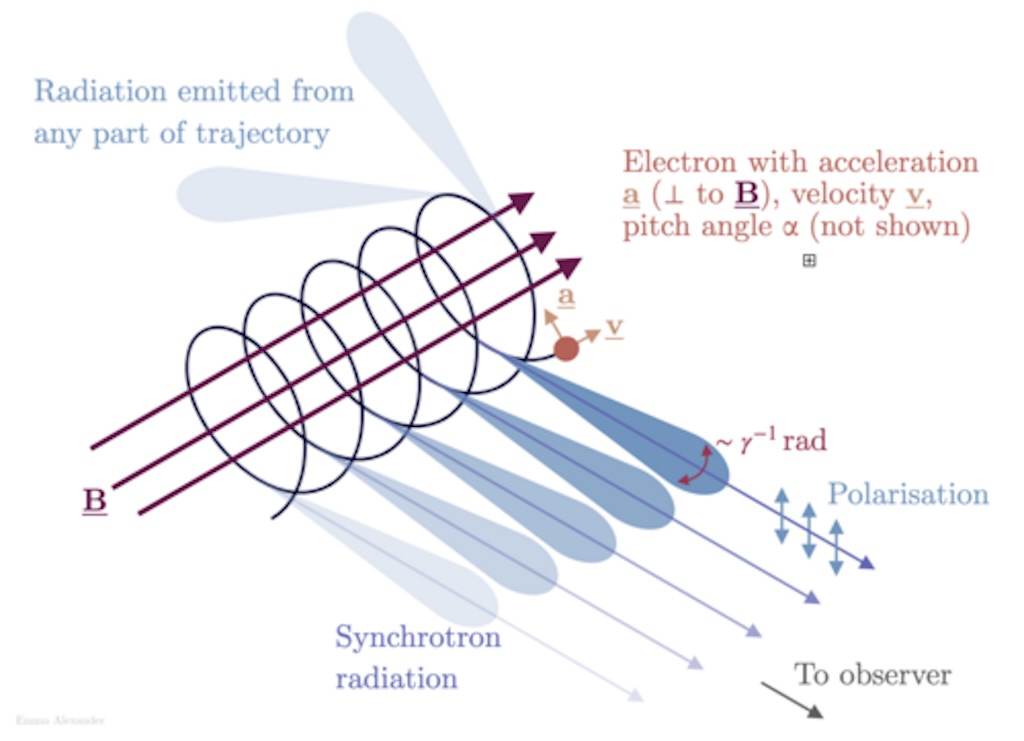
The situation is more complicated in astrophysical objects where the particle energy is relativistic (i.e. their speed approaches the speed of light). In this case, the radiation is compressed into a small range of angles (blue cones) around the instantaneous velocity vector of the particle. This is referred to as relativistic beaming, and it produces a broadened emission spectrum whose detailed shape depends on the particle momentum perpendicular to the magnetic field. Even in this regime, there remains a maximum photon energy that can be radiated, which is proportional to the field strength and inversely proportional to the particle momentum.
In radio astronomy, this emission is commonly produced by relativistic electrons accelerated in magnetic fields, for example through synchrotron radiation. Such radiation is often strongly linearly polarised. Here, polarisation does not refer to the beaming angles, but to the preferred orientation of the electric field oscillation in the emitted wave. The observed polarisation direction is determined by the component of the magnetic field perpendicular to the line of sight, and therefore provides a direct diagnostic of the magnetic field geometry and degree of ordering within the radio-emitting region.
An active galactic nucleus (AGN) is a compact region at the center of a galaxy that emits a significant amount of energy across the electromagnetic spectrum (including radio), with characteristics indicating that this luminosity is not produced by the stars. Active galactic nuclei are the most luminous persistent sources of electromagnetic radiation in the universe, and the observed characteristics of an AGN depend on several properties such as the mass of the central black hole, the rate of gas accretion onto the black hole, the orientation of the accretion disk, the degree of obscuration of the nucleus by dust, and presence or absence of jets. Numerous subclasses of AGN have been defined on the basis of their observed characteristics; the most powerful AGN are classified as quasars. A blazar is an AGN with a jet pointed toward the Earth, in which radiation from the jet is enhanced by relativistic beaming.
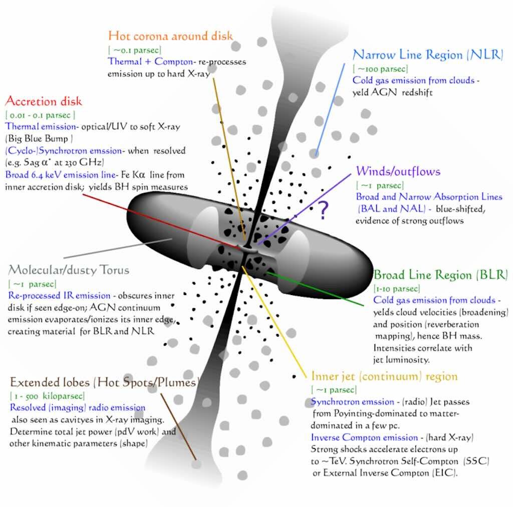
I include below a far more complex view of how the unified AGN model explains the spectral features of these objects. Note the multi-scale structure, spanning several order of magnitudes in size (image not to scale). The colour coding differentiate the structures, where order-of-magnitude estimates of the structures’ scale are indicated in light green, and the spectral features (mostly emission) are highlighted in blue. This is taken from the thesis work of Salvo Cielo in Numerical Models of AGN Feedback.
Here are a few more videos about the general topic of radio telescopes:-
Lovell Lecture: Professor Tim O’Brien accessible introduction, but often with a different more practical focus (less scientific) than the earlier videos, using the telescopes at Jodrell Bank.
China’s Giant Radio Telescope That Can Hear the Universe is a very accessible description of Five-hundred-meter Aperture Spherical Telescope (FAST), including how it was built.
How Engineers Built the Largest & Most Sensitive Radio Telescope on the Planet is also an accessible introduction to FAST, and how it was built, but set in a more extensive historical context.
Interferometres
An astronomical interferometer is a set of separate telescopes, mirror segments, or radio telescope antennas that work together as a single telescope to provide higher resolution images of astronomical objects such as stars, nebulas and galaxies by means of interferometry. The advantage of this technique is that it can theoretically produce images with the angular resolution of a huge telescope with an aperture equal to the separation, called baseline, between the component telescopes.
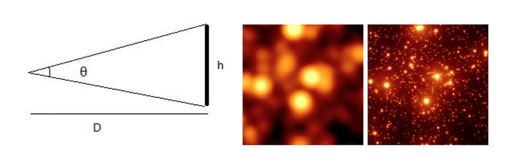
In astronomical measurements the distance to the objects being observed is generally unknown. This means that we can only measure sizes in terms of angular size θ, the fraction of a circle measured in angular units. The Moon and Sun both have angular diameters of about half a degree. The degree is rather large compared to the angular size of most astronomical objects, so smaller units are also commonly used, for example the arcsecond, which is 1/3600th of a degree. The angular size of the planet Saturn as seen from Earth averages about 17 arcseconds, with some variation as the planets’ relative distance changes with their orbits about the Sun. Galaxies seen halfway across the visible universe are about 1012 times larger in radius than Saturn and are further away by roughly the same factor, so they have an angular size of a few arcseconds.
The spatial resolution of a ground-based visible-light telescope is roughly one arcsecond. Many astronomical sources of radiation have angular sizes far smaller than this: the nearest star to the Sun, Proxima Centauri, has an angular size of about 1 milli-arcsecond. A object whose angular size is smaller than the resolution of the telescope being used is described as being unresolved.
So angular size is the size of the object’s image on the sky. Angular resolution is the smallest detail your telescope can separate. An object is resolved only when its angular size is larger than the telescope’s resolution. If the object is bigger than the telescope’s resolution, you see structure. If it is smaller, you only see a point of light.
Remember angular resolution is the smallest angle on the sky that the telescope can distinguish. Whereas spatial resolution is the actual physical size you can distinguish at the object.
Above we see a telescope equipped with a mirror, and we see the observed image from a point-like star as a dot of light, with the Airy disk. Unfortunately, the Airy disk does not contain any information relative to the star, irrespective of its size, shape, effective temperature, luminosity, distance, etc. A larger telescope with a larger diameter mirror, would lead to a smaller Airy disk for the star being imaged, providing a slightly better angular resolution image but with no more specific information related to the star.
Observing an extended celestial source (a distant resolved Earth-like planet as shown), more details are seen with the telescope having a larger diameter.
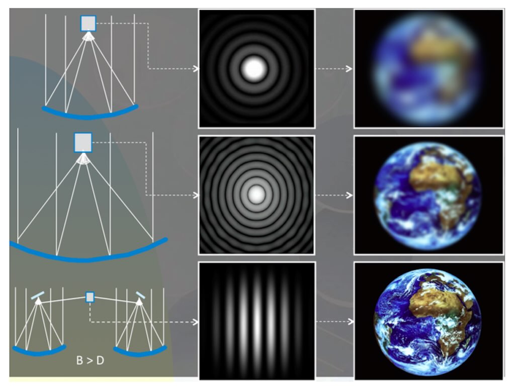
It was already in 1868 that Hippolyte Fizeau (1819-1896) and Édouard Stephan (1837-1923) realised that the angular resolution of two small apertures of a certain distance apart are equivalent to a single large aperture of that same distance. It is possible to reconstruct high angular resolution images of a distant celestial source using interferometers. In fact, the image of a distant star that one would see in the focal plane of a Fizeau-type interferometer is no longer just an Airy disk due to each single telescope aperture but a brighter Airy disk superimposed with a series of interference fringes, alternately bright and dark, perpendicularly oriented with respect to the line joining the two telescopes. Now we can see the improvement in angular resolution for our extended celestial source, firstly by increasing the diameter of the mirror, and then with an interferometer composed of two telescopes separated by a distance greater than the diameter of the mirrors.
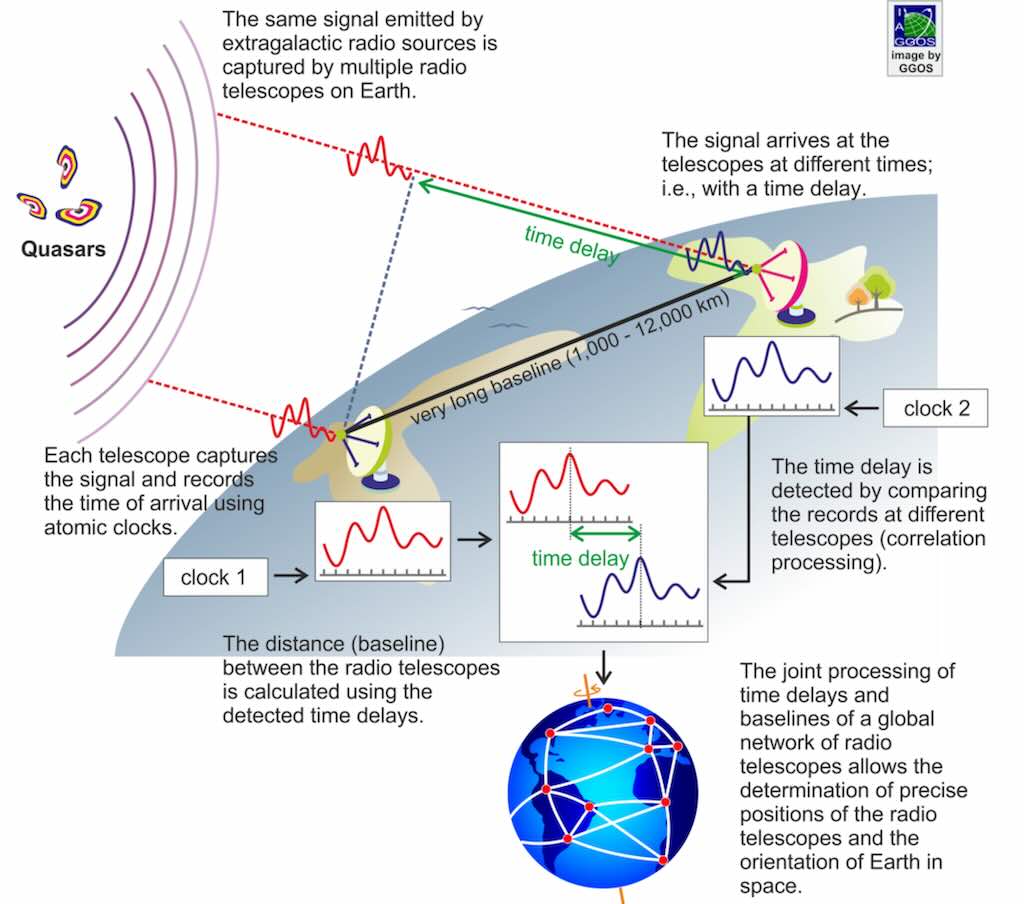
Interferometry is most widely used in radio astronomy, in which signals from separate radio telescopes are combined. A mathematical signal processing technique called aperture synthesis is used to combine the separate signals to create high-resolution images. In Very Long Baseline Interferometry (VLBI) radio telescopes separated by thousands of kilometers are combined to form a radio interferometer with a resolution which would be given by a hypothetical single dish with an aperture thousands of kilometers in diameter.
Mapping the radio sky
Aperture synthesis is a type of interferometry that mixes signals from a collection of telescopes to produce images having the same angular resolution as an instrument the size of the entire collection. At each separation and orientation, the lobe-pattern of the interferometer produces an output which is one component of the Fourier transform of the spatial distribution of the brightness of the observed object. The image (or “map”) of the source is produced from these measurements. Astronomical interferometers are commonly used for high-resolution optical, infrared, submillimetre and radio astronomy observations.
Earth Rotation Synthesis is a short video describing how the rotation of the earth is used in radio interferometers to change the orientation of arrays of antennas to generate new information for imaging the sky.
A visit to the Very Large Array near Magdalena, New Mexico is a simple look at the VLA (now named the JVLA), and this video is One Whole Day at the Very Large Array (drone flyover, no commentary).
Quasars
Large Quasar Groups is a video describing what a quasar is, and the fact that its discovery forced science to reconsider some of the most fundamental assumptions of cosmology. It includes a historical review of discovery of the pulsar. It is one of the best videos on radio astronomy I’ve seen.
Distant Quasars: Shedding Light on Black Holes is a video about how scientists study a faraway black hole that emits no light? Researchers use a “galaxy-sized lens” to analyse light from a distant quasar, revealing a supermassive black hole.
A quasar is an extremely luminous active galactic nucleus (AGN). The emission from an AGN is powered by accretion onto a supermassive black hole with a mass ranging from millions to tens of billions of solar masses, surrounded by a gaseous accretion disc. Gas in the disc falling towards the black hole heats up and releases energy in the form of electromagnetic radiation. The radiant energyof quasars is enormous; the most powerful quasars have luminosities thousands of times greater than that of a galaxy such as the Milky Way.
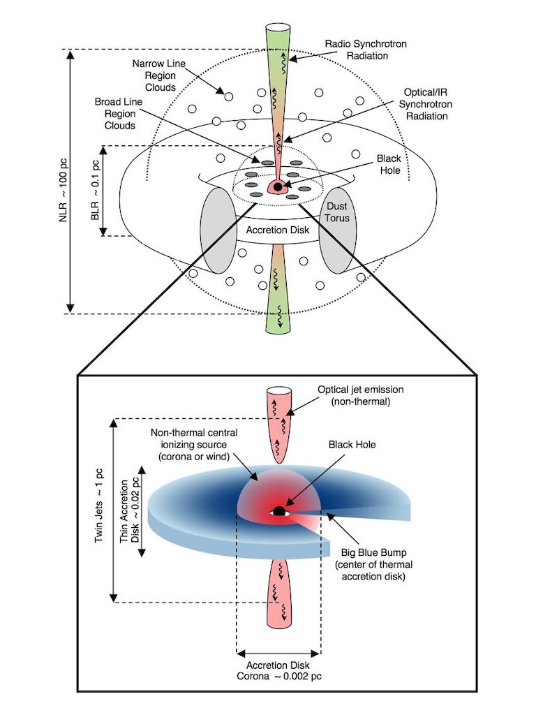
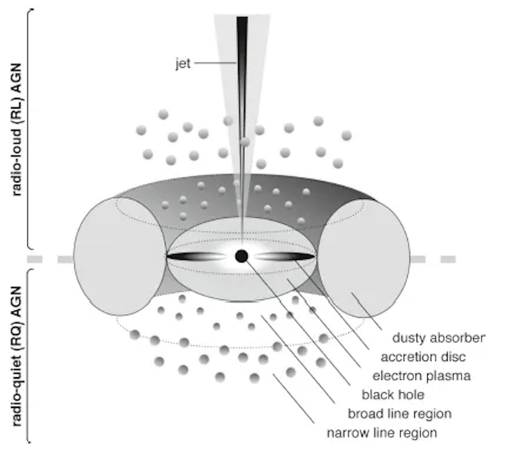
Above is a schematic diagram of the structure of a typical quasar. The upper part is on scales from 0.002 − 100 pc (a pc is a parsec or 3.26 light-years, or about 31 trillion kilometres) or from 6×10¹⁰ km to 3.1×10¹⁵ km.
The main components are the broad and narrow-line emission clouds and a dust torus that obscures the black hole in certain orientations. In radio-loud quasars, powerful (and often relativistic) jets are ejected from the central engine. These jets emit over the entire electromagnetic spectrum, with optical/IR dominating on scales 0.1 pc, and radio emission dominating on larger scales.
In the lower diagram, on scales 1 pc, a geometrically thin disk forms around the massive accreting black hole. In some quasars, the innermost portion of the accretion disk is seen as the ‘big blue bump’. All quasars also have a source of non-thermal emission, a corona, which dominates in the red, and produces enough UV radiation to ionise the broad and even narrow line regions. In radio-loud quasars, the base of the jet also will produce a non-thermal, typically highly-variable, red emission that can outshine the central corona.
The first quasars (3C 48 and 3C 273) were discovered in the late 1950s, as radio sources in all-sky radio surveys. They were first noted as radio sources with no corresponding visible object. Using small telescopes and the Lovell Telescope as an interferometer, they were shown to have a very small angular size. By 1960, hundreds of these objects had been recorded, and in 1963, a definite identification of the radio source 3C 48 with an optical object was found. Astronomers had detected what appeared to be a faint blue star at the location of the radio source and obtained its spectrum, which contained many unknown broad emission lines. The anomalous spectrum defied interpretation.
Another radio source, 3C 273 had a visible counterpart, and the spectrum also revealed the same strange emission lines. Finally it was thought that these were likely to be the ordinary spectral lines of hydrogen redshifted by 15.8%. At the time, this was a high redshift, since only a handful of much fainter galaxies were known to have a higher redshift. If this was due to the physical motion of the “star”, then 3C 273 was receding at an enormous velocity, around 47,000 km/s, far beyond the speed of any known star and defying any obvious explanation. Nor would an extreme velocity help to explain 3C 273’s huge radio emissions. If the redshift was cosmological (now known to be correct), the large distance implied that 3C 273 was far more luminous than any galaxy, but much more compact. Also, 3C 273 was bright enough to detect on archival photographs dating back to the 1900s, and it was found to be variable on yearly timescales, implying that a substantial fraction of the light was emitted from a region less than 1 light-year in size, tiny compared to a galaxy.
The strange spectrum of 3C 48 was quickly identified as hydrogen and magnesium redshifted by 37%. Shortly afterwards, two more quasar spectra in 1964 and five more in 1965 were also confirmed as ordinary light that had been redshifted to an extreme degree.
An extreme redshift could imply great distance and velocity but could also be due to extreme mass or some unknown law of nature. Extreme velocity and distance would also imply immense power output, which lacked explanation. The small sizes were confirmed by interferometry and by observing how quickly the quasar as a whole varied in output, and by their inability to be seen with even the most powerful visible-light telescopes as anything more than faint, starlike points of light. However, if they were small and far away, their power output would have to be immense for their size, making them difficult to explain. Equally, if they were very small and much closer to this galaxy, it would be easy to explain their apparent power output, but less easy to explain their redshifts and lack of detectable movement against the background of the universe.
Redshift is also associated with the expansion of the universe, as codified in Hubble’s law. If the measured redshift was due to relative velocity caused by inflation, then this would support an interpretation of very distant objects with extraordinarily high luminosity and power output, far beyond any object observed to date. This extreme luminosity would also explain the large radio signal. So 3C 273 could either be an individual star around 10 km wide within (or near to) this galaxy, or a distant active galactic nucleus. A distant and extremely powerful objects seemed more likely to be correct.
This explanation for the high redshift was not widely accepted at the time. A major concern was the enormous amount of energy these objects would have to be radiating, if they were distant. In the 1960s no commonly accepted mechanism could account for this. The currently accepted explanation, that it is due to matter in an accretion disc falling into a supermassive black hole, was only suggested in 1964 by Edwin E. Salpeter and Yakov Zeldovich, and even then it was rejected by many astronomers, as at this time the existence of black holes at all was widely seen as theoretical.
Various explanations were proposed during the 1960s and 1970s, each with their own problems. It was suggested that quasars were nearby objects, and that their redshift was not due to the expansion of space but rather to light escaping a deep gravitational well. This would require a massive object, which would also explain the high luminosities. However, a star of sufficient mass to produce the measured redshift would be unstable and in excess of the Hayashi limit. Quasars also show forbidden spectral emission lines, previously only seen in hot gaseous nebulae of low density, which would be too diffuse to both generate the observed power and fit within a deep gravitational well. There were also serious concerns regarding the idea of cosmologically distant quasars. One strong argument against them was that they implied energies that were far in excess of known energy conversion processes, including nuclear fusion. There were suggestions that quasars were made of some hitherto unknown stable form of antimatter in similarly unknown types of region of space, and that this might account for their brightness. Others speculated that quasars were a white hole end of a wormhole, or a chain reaction of numerous supernovae.
Eventually, starting from about the 1970s, many lines of evidence (including the first X-ray space observatories, knowledge of black holes and modern models of cosmology) gradually demonstrated that the quasar redshifts are genuine and due to the expansion of space, that quasars are in fact as powerful and as originally suggested, and that their energy source is matter from an accretion disc falling onto a supermassive black hole. This included crucial evidence from optical and X-ray viewing of quasar host galaxies, finding of “intervening” absorption lines, which explained various spectral anomalies, and observations from gravitational lensing.
This model also fits well with other observations suggesting that many or even most galaxies have a massive central black hole. It would also explain why quasars are more common in the early universe. As a quasar draws matter from its accretion disc, there comes a point when there is less matter nearby, and energy production falls off or ceases, as the quasar becomes a more ordinary type of galaxy.
The accretion-disc energy-production mechanism was finally modeled in the 1970s, and black holes were also directly detected (including evidence showing that supermassive black holes could be found at the centers of this and many other galaxies), which resolved the concern that quasars were too luminous to be a result of very distant objects or that a suitable mechanism could not be confirmed to exist in nature. By 1987 it was “well accepted” that this was the correct explanation for quasars, and the cosmological distance and energy output of quasars was accepted by almost all researchers.
Supermassive black holes and their jets
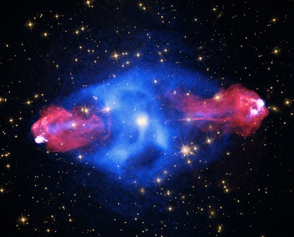
There is nothing better than to see what the VLA sees. And above we have the X-ray, optical & radio images of Cygnus A. This galaxy, at a distance of some 700 million light years, contains a giant bubble filled with hot, X-ray emitting gas (blue). Radio data from the Very Large Array (red) reveal “hot spots” about 300,000 light years out from the centre of the galaxy where powerful jets emanating from the galaxy’s supermassive black hole end. The visible light data is in yellow.
Visualises the scale of the smallest and largest black holes is an excellent video to describing the sizes and scales of black holes, etc,
Radiation from quasars is partially “nonthermal” (i.e., not due to black-body radiation), and approximately 10% are observed to also have jets and lobes like those of radio galaxies which also carry significant (but poorly understood) amounts of energy in the form of particles moving at relativistic speeds. Extremely high energies might be explained by several mechanisms (see Fermi acceleration and Centrifugal mechanism of acceleration). Quasars can be detected over the entire observable electromagnetic spectrum, including radio, infrared, visible light, ultraviolet, X-ray and even gamma rays. Most quasars are brightest in their rest-frame ultraviolet wavelength of 121.6 nm Lyman-alpha emission line of hydrogen, but due to the tremendous redshifts of these sources, that peak luminosity has been observed as far to the red as 900.0 nm, in the near infrared. A minority of quasars show strong radio emission, which is generated by jets of matter moving close to the speed of light. When viewed downward, these appear as blazars and often have regions that seem to move away from the centre faster than the speed of light (superluminal expansion). This is an optical illusion due to the properties of special relativity.
A supermassive black hole (SMBH) is the largest type of black hole, with its mass being on the order of hundreds of thousands, or millions to billions, of times the mass of the Sun. Black holes are a class of astronomical objects that have undergone gravitational collapse, leaving behind spheroidal regions of space that nothing, not even light, can escape. Observational evidence indicates that almost every large galaxy has a supermassive black hole at its centre. For example, the Milky Way galaxy has a supermassive black hole at its centre, corresponding to the radio source Sagittarius A*. Accretion of interstellar gas onto supermassive black holes is the process responsible for powering active galactic nuclei (AGNs) and quasars.
In 1967 it was suggested that nearly all sources of extra-galactic radio emission could be explained by a model in which particles are ejected from galaxies at relativistic velocities, meaning they are moving near the speed of light, and the compact central nucleus could be the original energy source for these relativistic jets.
Relativistic jets are beams of ionised matter accelerated close to the speed of light. Most have been observationally associated with central black holes of some active galaxies, radio galaxies or quasars, and also by galactic stellar black holes, neutron stars or pulsars. Beam lengths may extend between several thousand, hundreds of thousands or millions of parsecs. Jet velocities when approaching the speed of light show significant effects of the special theory of relativity; for example, relativistic beaming that changes the apparent beam brightness.
Massive central black holes in galaxies have the most powerful jets, but their structure and behaviours are similar to those of smaller galactic neutron stars and black holes. These SMBH systems are often called microquasars and show a large range of velocities. SS 433 jet, for example, has a mean velocity of 0.26c. Relativistic jet formation may also explain observed gamma-ray bursts, which have the most relativistic jets known, being ultrarelativistic.
Mechanisms behind the composition of jets remain uncertain, though some studies favour models where jets are composed of an electrically neutral mixture of nuclei, electrons, and positrons, while others are consistent with jets composed of positron–electron plasma. Trace nuclei swept up in a relativistic positron–electron jet would be expected to have extremely high energy, as these heavier nuclei should attain velocity equal to the positron and electron velocity.
Quasars were originally ‘quasi-stellar’ in optical images, because they had optical luminosities that were greater than that of their host galaxy. They always show strong optical continuum emission, X-ray continuum emission, and broad and narrow optical emission lines. Some astronomers use the term QSO (Quasi-Stellar Object) for this class of AGN, reserving ‘quasar’ for radio-loud objects, while other astronomers talk about radio-quiet and radio-loud quasars. The host galaxies of quasars can be spirals, irregulars, or ellipticals. There is a correlation between the quasar’s luminosity and the mass of its host galaxy, in that the most luminous quasars inhabit the most massive galaxies (ellipticals).
There are several subtypes of radio-loud active galactic nuclei. Firstly, the radio-loud quasars that behave exactly like radio-quiet quasars with the addition of emission from a jet. Thus they show strong optical continuum emission, broad and narrow emission lines, and strong X-ray emission, together with nuclear and often extended radio emission. Then there are the “Blazars” (BL Lacertae (BL Lac) objects and optically violent variable (OVV) quasars) distinguished by rapidly variable, polarised optical, radio, and X-ray emissions. BL Lac objects show no optical emission lines, broad or narrow, so that their redshifts can only be determined from features in the spectra of their host galaxies. The emission-line features may be intrinsically absent, or simply swamped by the additional variable component. In the latter case, emission lines may become visible when the variable component is at a low level. OVV quasars behave more like standard radio-loud quasars with the addition of a rapidly variable component. In both classes of source, the variable emission is believed to originate in a relativistic jet that is oriented close to the line of sight. Relativistic effects amplify both the luminosity of the jet and the amplitude of variability. And finally, there are the radio galaxies that show nuclear and extended radio emission. Their other AGN properties are heterogeneous. They can broadly be divided into low-excitation and high-excitation classes. Low-excitation objects show no strong narrow or broad emission lines, and the emission lines they do have may be excited by a different mechanism. Their optical and X-ray nuclear emission is consistent with originating purely in a jet.
Key reminders:-
Quasars are accreting supermassive black holes. The enormous luminosity of a quasar does not come from the black hole itself. It comes from the accretion disk, where gas spirals inward, heats up, and radiates intensely.
The accretion disk is a plasma (super-hot free electrons and ions), threaded by magnetic fields. Gas cannot fall into a black hole unless it loses angular momentum, and the disk enables this through turbulence and effective viscosity. A rapidly rotating plasma disk, coupled to strong magnetic fields, also provides a natural mechanism for launching jets. This means magnetic forces can extract rotational energy, collimate outflows, and accelerate particles to relativistic speeds.
The jets are therefore like magnetically driven exhaust pipes. However, only about ~10% of quasars are radio-loud, producing the most powerful large-scale jets.
Gravitational lensing
A gravitational lens is matter, such as a cluster of galaxies or a point particle, that bends light from a distant source as it travels toward an observer. The amount of gravitational lensing is described by Albert Einstein‘s general theory of relativity.
Unlike an optical lens, a point-like gravitational lens produces a maximum deflection of light that passes closest to its center, and a minimum deflection of light that travels furthest from its center. Consequently, a gravitational lens has no single focal point, but a focal line. If the (light) source, the massive lensing object, and the observer lie in a straight line, the original light source will appear as a ring around the massive lensing object (provided the lens has circular symmetry). If there is any misalignment, the observer will see an arc segment instead.
There are three classes of gravitational lensing. Firstly, strong lensing is where there are easily visible distortions such as the formation of Einstein rings, arcs, and multiple images. Then weak lensing is where the distortions of background sources are much smaller and can only be detected by analyzing large numbers of sources in a statistical way to find coherent distortions of only a few percent. And microlensing is where no distortion in shape can be seen but the amount of light received from a background object changes in time.
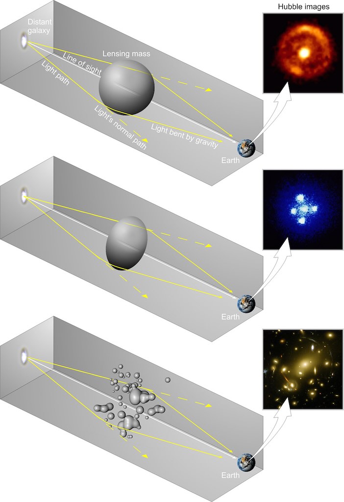
Depending on the shape of the intervening object, gravitational lensing can produce rings, Einstein crosses or arcs.
Gravitational Lensing is a really useful video description.
Pulsars
Signals from the first discovered pulsar were initially observed by Jocelyn Bell while analysing data recorded on August 6, 1967, from the newly commissioned Interplanetary Scintillation Array that she helped build. Initially dismissed as radio interference by her supervisor and developer of the telescope, Antony Hewish, the fact that the signals always appeared at the same declination and right ascension soon ruled out a terrestrial source. On November 28, 1967, Bell and Hewish using a fast strip chart recorder resolved the signals as a series of pulses, evenly spaced every 1.337 seconds. No astronomical object of this nature had ever been observed before. Then a second pulsating source CP 1919 was discovered in a different part of the sky. Although CP 1919 emits in radio wavelengths, pulsars have subsequently been found to emit in visible light, X-ray, and gamma ray wavelengths. A pulsar is analogous to the “twinkling” of stars due to the passage of light through the Earth’s atmosphere (planets don’t twinkle).
In 1974, Joseph Hooton Taylor, Jr. and Russell Hulse discovered for the first time a pulsar in a binary system of stars. This pulsar orbits another neutron star with an orbital period of just eight hours. Einstein‘s theory of general relativity predicts that this system should emit strong gravitational radiation, causing the orbit to continually contract as it loses orbital energy. Observations of the pulsar soon confirmed this prediction, providing the first ever evidence of the existence of gravitational waves.
In 1992, Aleksander Wolszczan discovered the first extrasolar planets around a pulsar, 2,300 light-years from the Sun, in the constellation Virgo. The pulsar has a planetary system with three known pulsar planets. So they were both the first extrasolar planets to be discovered and the first pulsar planets to be discovered. This discovery presented important evidence concerning the widespread existence of planets outside the Solar System, although it is very unlikely that any life form could survive in the environment of intense radiation near a pulsar.
The existence of neutron stars (gravitationally collapsed core of a massive supergiant star) was first proposed by Walter Baade and Fritz Zwicky in 1934, when they argued that a small, dense star consisting primarily of neutrons would result from a supernova. Based on the idea of magnetic flux conservation from magnetic main sequence stars, Lodewijk Woltjer proposed in 1964 that such neutron stars might contain massive magnetic fields. In 1967, shortly before the discovery of pulsars, Franco Pacini suggested that a rotating neutron star with a magnetic field would emit radiation, and even noted that such energy could be pumped into a supernova remnant around a neutron star. After the discovery of the first pulsar, Thomas Gold independently suggested a rotating neutron star model similar to that of Pacini, and explicitly argued that this model could explain the pulsed radiation observed by Bell Burnell and Hewish. In 1968, Richard V. E. Lovelace with collaborators, discovered the period of approximately 33 ms of the Crab Nebula Pulsar. This confirmed the rotating neutron star model of pulsars.
Pulsar astronomy & data analysis using MeerKAT is a great video tutorial on pulsars.
Checkout the technical description below…
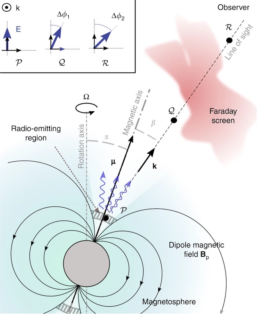
The above diagram ties to illustrate the basic geometric model of radio emission and polarisation in a pulsar magnetosphere. A pulsar is a rapidly rotating neutron star whose strong dipolar magnetic field Bp channels charged particles along curved field lines. Radio emission is produced in a localised region above the magnetic pole, where coherent radiation is generated and escapes along the local propagation direction k.
Because the magnetic axis is generally tilted with respect to the rotation axis, the emission beam sweeps through space as the star rotates with angular velocity Ω. An observer detects a pulse whenever the line of sight intersects the radio beam. The angles α and β describe the inclination of the magnetic axis relative to the rotation axis and the observer’s closest approach to the magnetic axis, respectively.
The diagram also shows how the observed polarisation is modified during propagation. The emitted wave passes through a magnetised plasma “Faraday screen”, which rotates the plane of linear polarisation by an amount Δϕ. The inset illustrates how the electric field vector E changes between points P, Q, and R, producing a measurable polarisation rotation. Such effects allow radio astronomers to probe both the pulsar’s magnetic geometry and the intervening plasma along the line of sight.
Another telescope with no moving parts
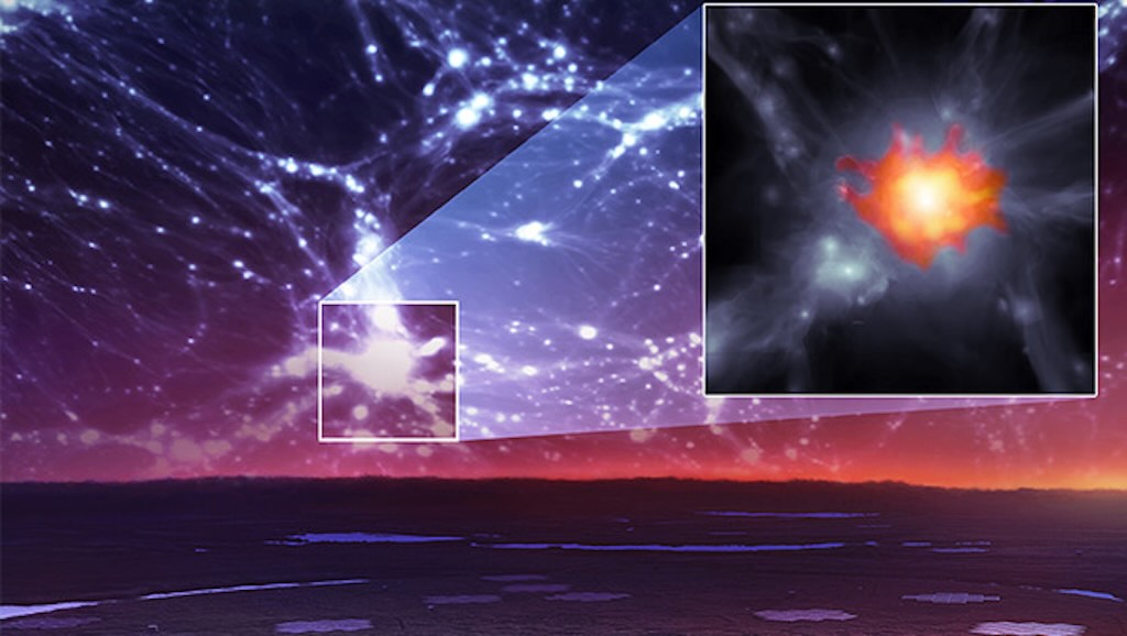
An artist’s impression of the vast space of the universe above the LOFAR telescope, with the inset shows a magnified image of a galaxy cluster where a megahalo is being observed with LOFAR.
The Low-Frequency Array (LOFAR at www.astron.nl) is a next-generation software radio interferometer optimised for astrophysical observations at long metre wavelengths (~10–240 MHz), corresponding to radio frequencies largely unexplored with high sensitivity before its commissioning. LOFAR exemplifies a shift from traditional dish-based telescopes to digitally steered phased arrays of simple antennas.
LOFAR’s fundamental sensors are dipole antenna elements, split into low-band (~10–80 MHz) and high-band (~110–240 MHz). These broad-band elements lack mechanical pointing, relying instead on digital beam-forming to select sky directions electronically.
The antennas are grouped into ~52 stations distributed across Europe, with the majority in the Netherlands. By connecting these stations with high-speed optical links to a central correlator in Groningen, the array achieves interferometric baselines exceeding 1000 km, giving arc-second class angular resolution at the highest frequencies. Digitisation and initial signal conditioning occur at each station. Central processing uses a GPU-accelerated correlator and beamformer (COBALT) to combine signals across the array, producing calibrated visibilities and multiple simultaneous beams, producing time-domain (transient) surveys alongside deep imaging.
The combination of large collecting area, extensive baselines, and digital flexibility makes LOFAR a software-defined telescope, where spatial resolution, field of view, and observing modes are set by processing rather than mechanical steering.
The LOFAR Two-metre Sky Survey (LoTSS) and its Deep Fields are among the most ambitious low-frequency imaging programs ever undertaken. Such deep images reveal star-forming galaxies (SFGs) over a broad range of cosmic epochs, including dust-obscured systems inaccessible to optical surveys. Because radio continuum at these frequencies traces non-thermal synchrotron emission from cosmic rays accelerated in supernova remnants, it provides an unbiased star-formation tracer largely independent of dust extinction.
LOFAR has uncovered remarkable systems such as giant radio galaxies with lobes spanning tens of millions of light-years, probing AGN feedback and magnetic field evolution over vast scales.
Though technically challenging due to foreground contamination, LOFAR continues to seek redshifted 21 cm emission from neutral hydrogen in the early Universe (value of a redshift is often denoted by the letter z, and z~6–11 means a Universe from about 0.9–1.0 billion years old down to about 0.4 billion years old). This offers a path to understanding cosmic reionisation, the process that caused electrically neutral atoms in the primordial universe to reionise after the lapse of the “dark ages“.
Probing the cold Universe
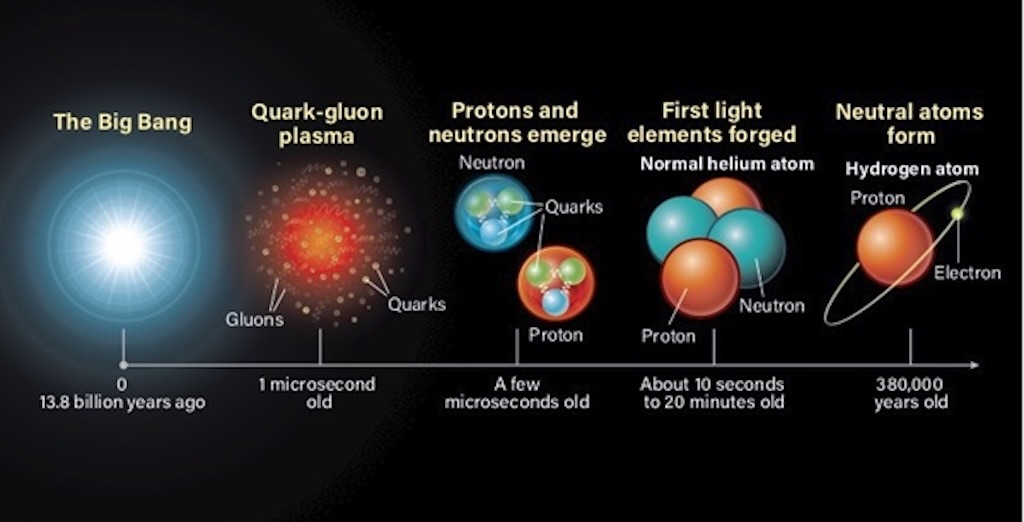
The title mention a “cold” Universe which is not about the heat death of the universe, but about being “cold” because hydrogen gas is not highly excited, as shown in its hydrogen spectral lines. This neutral hydrogen constitutes the dominant baryonic mass (protons and neutrons) component of the interstellar medium and represents the raw material from which molecular clouds and ultimately stars form.
The video a new all-sky survey of neutral hydrogen visualises the cold gaseous substrate from which stars are born. It’s the structural backbone of the Milky Way’s interstellar medium. The animation shows the full-sky distribution of neutral atomic hydrogen (HI) in the Milky Way, mapped via its 21-centimeter hyperfine emission line at 1420.4058 MHz. Firstly, the 21 cm line arises from the magnetic dipole “spin-flip” transition between the parallel and anti-parallel configurations of the electron and proton spins in the hydrogen ground state. Because 21 cm radiation penetrates interstellar dust, it allows us to map the Galactic gas disk independent of optical extinction.
Hydrogen produces different spectral features depending on its physical state, either cold neutral hydrogen (H I), warm ionised hydrogen (H II which would be just a free proton), or hot plasma. And temperature controls which energy levels are populated, and therefore which lines appear.
H I and H II are just a standard spectroscopic convention for electron states, where I means a neutral atom (no electrons removed), and II means a singly ionised atom (one electron removed).
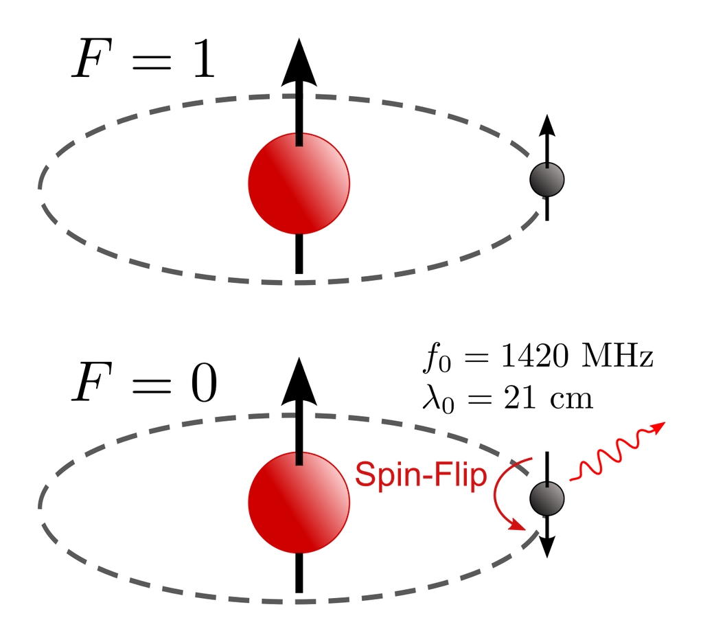
The main hydrogen line linked to the “cold universe” is the hydrogen hyperfine line at the wavelength 21.106 cm (1420.405 MHz frequency). It is produced by a spin-flip transition, which means the direction of the electron’s spin is reversed relative to the spin of the proton. This is a quantum state change (a relaxation) between the two hyperfine levels of the hydrogen 1 s ground state. And the resulting in emission of a photon with a 21 cm wavelength. This is not an ionisation (loss of an electron), it is simply a relaxation of neutral H I.
Hyperfine structure is defined by small shifts in otherwise degenerate electronic energy levels and the resulting splittings in those electronic energy levels, due to electromagnetic multipole interaction between the nucleus and electron clouds.
A single hydrogen atom has an extremely low probability of emitting this photon, i.e. average lifetime ~10 million years. But space contains astronomical quantities of hydrogen so the combined emission becomes strong. And because neutral hydrogen is everywhere. This line is like a “marker” and tells us if there are gas clouds in the Milky Way, what structure it has (spiral), if there is hydrogen between galaxies, and even what the early Universe looked like before stars existed. And these radio waves (photons) travel enormous distances, are not blocked like visible light (photons), and even pass through all types of dust.
Remember our 21 cm (210,000 micrometres) hydrogen photon is vastly larger than dust grains (~0.1 micrometres), so dust cannot scatter it efficiently. Whilst a light photon (~0.5 micrometres) will be easily scattered and absorbed.
The physics of molecular hydrogen in space with JWST is an excellent, in-depth, video introduction.
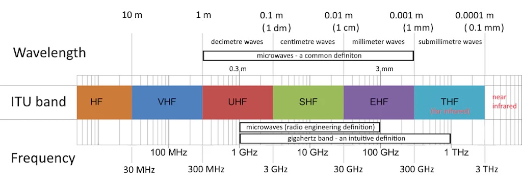
Sub-millimetre astronomy is another the branch of observational astronomy that is conducted at sub-millimetre wavelengths (i.e. terahertz radiation) of the electromagnetic spectrum. Astronomers place the sub-millimetre waveband between the far-infrared and microwave wavebands, typically taken to be between a few hundred micrometres and a millimetre. Sub-millimetre observations can be used to trace emission from gas and dust, including the C I and C II lines (respectively a neutral carbon atom neutral carbon with 6 electrons, and a singly ionised carbon with 5 electrons), and the lines of CO (carbon-monoxide).
In the millimetre (30–300 GHz) band you find adaptive cruise control and collision avoidance radar (76–81 GHz), airport body scanners (~24 GHz or ~70–80 GHz), 5G smartphone 5G in US is ≈24–40 GHz (but in Europe its only on 3.4–3.8 GHz, so not millimetre-wave). Sub-millimetre waves (300 GHz to 3 THz) is usually outside domestic use (but can include spectroscopy instruments). In astronomy, far-IR (0.3-10 THz) and sub-mm (0.3-3 THz) frequently overlap in terminology, with mid-IR covering warm dust (~100–1000 K) and far-IR/sub-mm for cold dust (~10–50 K), and millimetre is molecular rotational lines (CO, C I, etc.).
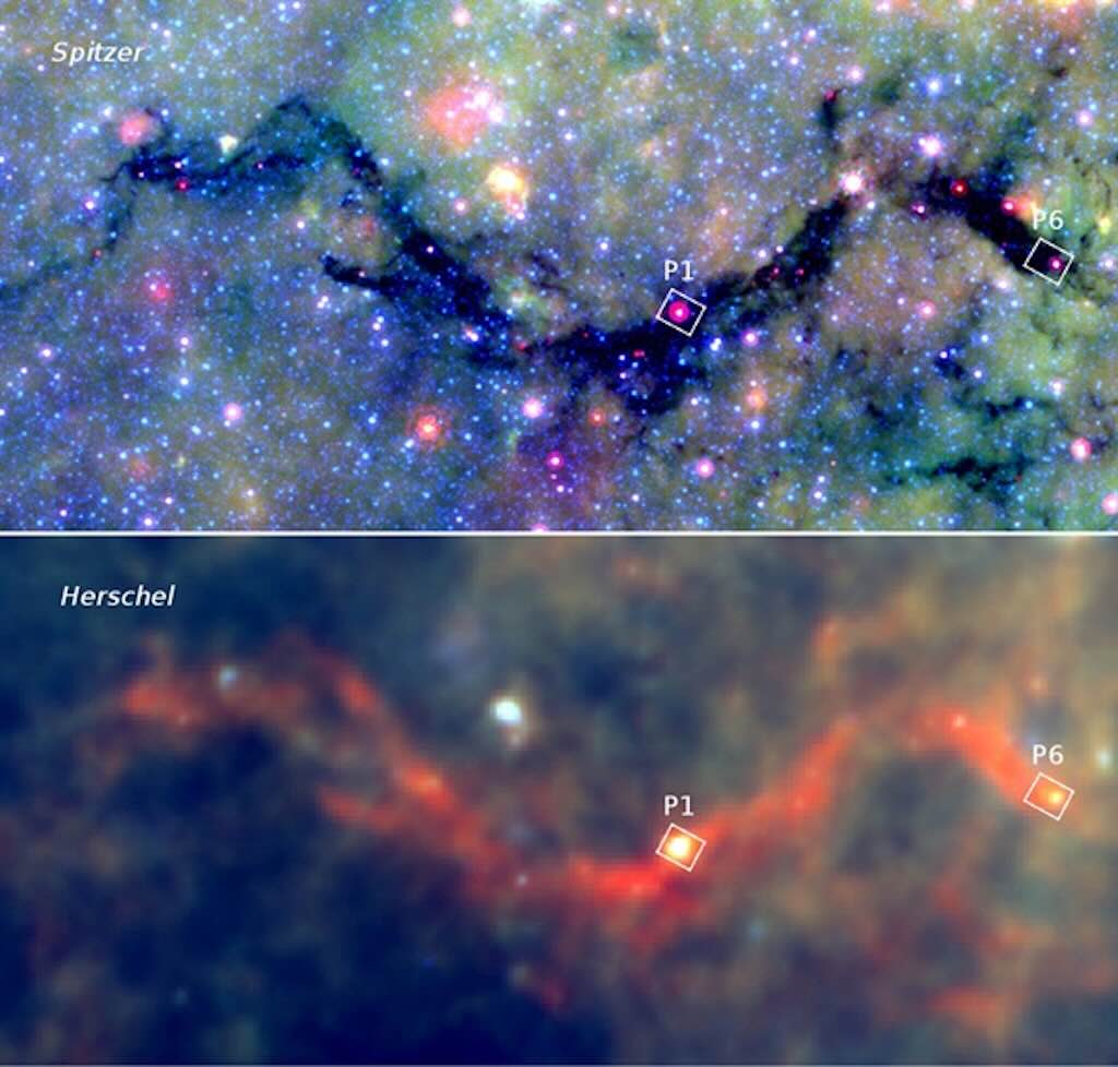
The two above panels show the Snake Nebula as photographed by the Spitzer and Herschel space telescopes.
The upper panel was taken by Spitzer which covers the mid- to far-infrared (~100 THz down to ~1.7 THz), and the thick nebular material blocks light from more distant stars.
The lower panel was taken by Herschel covers the far-infrared to sub-millimetre (~5.5 THz down to ~450 GHz), and we see the nebula glows due to emission from cold dust. The two boxed regions, P1 and P6, were examined in more detail by the Sub-millimeter Array.
An Introduction to Millimetre-Wave Astronomy is an accessible introduction video, with a focus on the Atacama Large Millimeter/Sub-millimeter Array.
A fantastic companion to the above video is When galaxies were born, a video by an excellent speaker, on the rich history of modern cosmology over the last 40 years. I found some of the comments particular useful as reminders, and I list them here:-
- The Big Bang was not a big explosion, with galaxies as projectiles expanding in to pre-existing space. They are actually “sitting on space” that is itself expanding (so not static but stretching).
- This meant that a blue light ray emitted from a galaxy, will take such a long time to get to Earth, that not only has space stretched, but the light ray itself has stretched, becoming a red light ray (i.e. the redshift).
- This is not the same as the frequency of an ambulances siren changing as it passes by. That can also happen in the Universe, because galaxies can have very small motions, which will be the doppler effect, but the effect of the expansion of the Universe is quite different and happens on a very large scale.
- To measure this expansion we use the “fingerprints” of hydrogen, carbon or oxygen, contained in the emission of a galaxy. If we know in the laboratory what that radiation looks like at rest, then we can measure how far those fingerprints have shifted, and that is the red shift. And this is the factor by which the Universe has expanded, since that light left the object (or how smaller the Universe was when that light was emitted).
- This red shift is then converted in to a “lookback time“, the age of the universe now, minus the age of the universe when a photon was emitted at a distant location.
- And the “cosmic dawn” (reionisation) is the first moment that starlight appears (370,000 years after the Big Bang. Video of the formation and evolution of the first stars and galaxies in a virtual universe similar to our own. This is a short simulation that begins just before cosmic dawn, when the universe is devoid of starlight, and runs to the epoch 550 million years after the Big Bang. You see stars forming, that then explode as supernovas, and the nuclear products that have been synthesised in those stars become pollutants in space, and form the next generation of stars. And this leads to the chemistry we know today (and to life as well).
- It’s interesting that it was only 60 years ago that that the redshift being observed hinted at a Universe that was at least 550 million years old. Now we can measure a redshift that points to the age of Universe at around 13.8 billion years.
- Another elegant technique enabled the observational astronomer to pick a (distant) galaxy to look at. The spectrum of a distant galaxy (faint might not mean distant) has a cut-off in its spectrum due to redshifted ultraviolet light being absorbed by the hydrogen gas between the stars. So the idea is to take a image with different coloured light filters (including the shorter wavelength ultraviolet), and if a galaxy disappeared with an ultraviolet light, but is still there with the other coloured filters, then it must be further away (because it is behind a cloud of hydrogen that has cut off the ultraviolet). So as a galaxy moves more to higher redshift and hence more distant objects, it disappears successively with each filter. So finding the colour filter where the galaxy disappears, given an approximate redshift, and hence an approximate lookback time to that galaxy.
Sources of sub-millimetre emission include molecular clouds and dark cloud cores, which can be used to clarify the process of star formation from earliest collapse to stellar birth, by determining chemical abundances in dark clouds and the cooling mechanisms for the molecules which comprise them.
You see sometimes reference to millimetre and sub-millimetre, but they are essentially the same thing because there is no physical boundary between them. It’s one continuous band, and the same molecules produce lines across both.
Like the infrared, the sub-millimetre atmosphere is dominated by numerous water vapour absorption bands and it is only through “windows” between these bands that observations are possible. The ideal sub-millimetre observing site is dry, cool, has stable weather conditions and is away from urban population centres. Only a handful of sites have been identified. They include Mauna Kea (Hawaii), the Llano de Chajnantor Observatory on the Atacama Plateau (Chile), the South Pole, and Hanle in India (the Himalayan site of the Indian Astronomical Observatory).
Check out the video Things to know when visiting the Mauna Kea Observatory Telescopes which is for those taking a private visit up there, and the video on the Atacama Large Millimetre Array, a more technical, but still accessible, description.
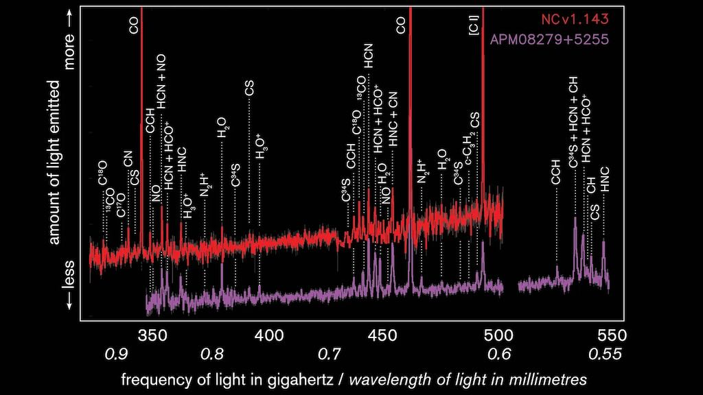
Let’s look at the above example. The figure presents a sub-millimetre spectral scan of two luminous extragalactic sources (not stars), plotted as emitted spectral intensity as a function of observing frequency. Two spectra are overlaid, NCv1.143 (red) and APM 08279+5255 (purple). The horizontal axis is labelled in frequency (GHz), spanning approximately 330–550 GHz, with the corresponding wavelength scale in millimetres indicated above (roughly 0.9–0.55 mm). This frequency range lies in the sub-millimetre regime of the electromagnetic spectrum.
The vertical axis represents the measured emission intensity (spectral brightness/flux density in relative units). The spectra consist of a continuum baseline with multiple superimposed emission features.
Before we look at what they are, let’s stop and think about how they were measured. The spectra are an excellent example of modern sub-millimetre engineering, site selection, calibration, and long integration time. Water vapour absorbs strongly in the sub-millimetre, so these were acquired over quite long periods with very low precipitable water vapour (PWV), e.g. in a mediocre night, much of this band would have been unusable. These are molecular emission lines from objects billions of light-years away, spread over large velocity widths, needing long integration times, and very low-noise receivers.
The front-end detectors are cooled to a few kelvin using cryogenics. The measured power levels are comparable to thermal noise in the receiver, so stability is everything. Unlike optical spectroscopy (gratings), sub-millimetre spectroscopy requires a local oscillator at hundreds of GHz, stable frequency references, and digital FFT spectrometers.
A dish that works at 21 cm can be rough, but a dish that works at 0.8 mm must be accurate to ~50 μm (the thickness of a human hair), across a 15–50 metre structure. The plot covers ~220 GHz of bandwidth, so the spectra would have been acquired over multiple tunings, repeated scans, and the stitching together of multiple parts of the spectrum.
Calibration would have required corrections for atmospheric transmission changes minute-to-minute, instrumental bandpass shape, sideband ambiguities (in heterodyne systems), and include an absolute flux calibration.
Unlike optical spectroscopy, where lines often arise from electronic transitions in atoms, sub-millimetre spectroscopy is dominated by molecular rotational structure and atomic fine-structure cooling lines.
So to be absolutely clear this type of spectrum is not related to the 21 cm H I hyperfine line (1.420 GHz). It lies at much higher frequencies and is dominated by molecular rotational and atomic fine-structure transitions rather than hyperfine emission from neutral hydrogen.
The spectra are characterised by a series of narrow emission peaks superimposed on a lower baseline level. Each peak corresponds to radiation emitted at a specific frequency by a quantised transition in an atom or molecule.
In the sub-millimetre regime, the dominant emission lines arise from rotational transitions of molecules (primarily CO and other dense-gas tracers) and fine-structure transitions of atoms or ions (notably neutral carbon). These transitions occur in cold and moderately warm interstellar gas (typical temperatures tens to hundreds of kelvin), where molecules and atoms populate low-lying rotational or fine-structure energy levels.
Several of the strongest labelled features are due to carbon monoxide (CO), the most commonly observed molecular tracer of cold molecular gas in galaxies. CO is a linear molecule with quantised rotational levels, where transitions occur between adjacent levels producing emission lines in the millimetre/sub-millimetre bands.
A sub-millimetre spectrum of this type provides a direct observational inventory of the emitting gas, allowing measurement of chemical composition (identified species), gas excitation and density (via line ratios), kinematics (via Doppler shifts and line profiles), and redshift and distance (through systematic displacement of line frequencies).
So this type of spectra permit the study of star formation conditions, interstellar chemistry, and how galaxies evolve across cosmic time,
Very long baseline interferometry
Very-long-baseline interferometry (VLBI) is a type of astronomical interferometry, and is best known for imaging distant cosmic radio sources. I understand it can also be used “in reverse” to perform Earth rotation studies, map movements of tectonic plates very precisely (within millimetres), and perform other types of geodesy.
Check out Developments in VLBI, which is very complete video.
The shadow of a black hole
The Event Horizon Telescope (EHT) combines data from several very-long-baseline interferometry (VLBI) stations around Earth, which form a combined array with an angular resolution sufficient to observe objects the size of a supermassive black hole‘s event horizon.
In 2019 they showed the first direct image of a black hole, which showed the supermassive black hole at the centre of Messier 87, designated M87*.
Event Horizon Telescope Animated Movie is useful, and Inside the black hole image that made history is a TED video.
The Event Horizon Telescope: Exploring the Cosmic Unknown Through Global Collaboration is a more complete video presentation.
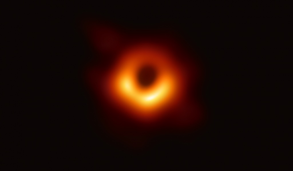
Above is the first image of a black hole in human history, captured by the Event Horizon Telescope, showing light emitted by matter as it swirls under the influence of intense gravity. This black hole is 6.5 billion times the mass of the Sun and resides at the centre of the galaxy M87.
The Square Kilometre Array
The Square Kilometre Array (SKA) is an intergovernmental international radio telescope project being built in Australia (low-frequency) and South Africa (mid-frequency). The name refers to the notional size of the telescope’s collecting area, not to the extent of the entire telescope array, which is far larger.
The Square Kilometre Array Telescope: Engineering to Reveal Cosmic Origins is a video about what is planned for 2027 and beyond.