Warning: This review is a work in progress
The Observable Universe
I had decided to follow an Oxford University Summer School (2026) on the subject “Exploring the Cosmos: Technology, Theory, and Discovery”.
One of the recommended reading was “Observational Astronomy” by Geoff Cottrell. It’s from the Oxford University Press, and is subtitled “A Very Short Introduction“.
I did not know this “very short” book series, but it would appear that there are over 800 titles published or announced. I was intrigued to see a revered academic publisher taking on such topics as American Politics (could quickly go out-of-date), Animal Rights, Elizabeth Bishop (who?), Polygamy, and Work (a nice combination).
I ordered the book and found it to be something like a Foolscap octavo (not A5 or A6) with a colourful durable coated cardstock, and a ~10-11 pt font. So it’s “very short” because it’s 154 pages are printed in a small font!
My guess is that the target for this pocket-format are readers 18 to 50 years old, with good eyesight, who waste time commuting on trains. I’m 74 and the font size will certainly be more tiring than a larger font.
I really dislike breaking the spine of even, zero self-respect, airport-fiction. But here I had no choice if I wanted to read the whole page. Once the spine broken, I felt I was allowed to deface the pages with abandon, which I did. Frankly, this is not the type of book I want seen sitting between my Feynman Lectures and my Oxford Companion to Western Art.
The Observable Universe
Somehow I felt that this first chapter was in many ways an introduction. It seemed to mention almost everything about the observable universe, including the bits you can’t see.
I’m not sure why, but I found the text dry and uninspiring. So I turned to the YouTube videos. On most topics I found a decent length video that I felt was authoritative, and in some cases professional prepared.
A Journey to the Edge of the Observable Universe (video)
“LIGO” Laser Interferometer Gravitational-wave Observatory (video)
Telescopes in Astronomy (video)
The largest telescope that will ever be built* (video introduction for the ELT in Paranal, Chile)
World’s Biggest Optical Telescope – ELT (video)
Exploring the Universe from La Palma with the Nordic Optical Telescope (video on optical telescope used to view gravitationally lensed quasars)
VISTA: A Pioneering New Survey Telescope Starts Work (video description of the Visible and Infrared Survey Telescope for Astronomy)
40 Years of Infrared Astronomy: Through the Eyes of IRAS (video)
Meet NASA’s Newest Set of X-ray Eyes on the Universe (video)
Exploring the Extreme Universe with the Fermi Gamma-ray Space Telescope (video)
How Engineers Built the Largest & Most Sensitive Radio Telescope on the Planet | Blueprint (video)
Journeys of Discovery: Jocelyn Bell Burnell and Pulsars (video history)
Surprise Find! Webb Telescope Uncovers Isolated Supermassive Quasars in Early Universe (video)
Galaxies (video)
A Star Explosion So Intense, It Compressed Earth’s Atmosphere from 2 Billion Light-Years Away (video)
Seeing Stars: The Curious History of Celestial Maps and the Conquest of Mars (video)
Pictures in the sky: the origin and history of the constellations (video)
History of The Telescope: From The Inventor Galileo to James Webb (video)
The Secret To Galileo’s Groundbreaking Telescope Revealed By Surprising Item | BBC Timestamp (video)
Why Humans Are Made Of Stars (video)
The Origin Of The Elements | Dr Stephen Wilkins (video)
A Beginner’s Guide to Black Holes – with Amélie Saintonge (video)
Supermassive Black Holes (video)
Uncovering the Secrets of the Sun (Full Episode) | National Geographic (video)
Almost touching stars – Astronomical Spectroscopy (video)
The Evolution of the Modern Milky Way Galaxy (video)
How Stars are Born | Hans Moritz Guenther | MIT IAP 2024 (video)
Battle of the Big Bang: New Theories Changing How We Understand the Universe (video)
We Might Be Wrong About the Force Pushing Our Universe Apart (video)
Telescopes
Fortunately the second chapter was far better structured, and the content a little easier to read. It was a very steep learning curve, however I could use the content to build a “note-taking”, as see below.
Start with the video “How the Telescope Changed Everything We Know About the Universe“.
In the background there is a source of all knowledge about Amateur Telescope Optics maintained by Vladimir Sacek. There are a lot of things in life that you just have to accept as true, because I’m simply not able to verify or validate its content. It covers in excruciating detail everything from early telescopes to atmospheric turbulence, to…
An optical telescope gathers and focuses light mainly from the visible part of the electromagnetic spectrum, to create a magnified image for direct visual inspection, to make a photograph, or to collect data through electronic image sensors.
Sources of noise in optical telescopes can be shot noise (associated with the particle nature of light), and thermal noise (from dark current and electronics).
The key is to increase signal-to-noise. This can be by using bigger mirrors, longer exposure times, stacked exposures, cooling to reduce dark current in sensors, use of low-noise electronics, use of narrow band filters, reduce light pollution, better mirror and lens coating, good baffling, clean optics, blackened interiors, pixel size optimisation, and using better sensors and post-processing.
I’m guessing it must be possible to use “bracketing” (or multiple exposure times or short and long integrations). This can be taking multiple exposures of the same target with different settings. High Dynamic Range (HDR) astronomy, e.g. exposure bracketing to avoid saturation, bracketing across filters (broadband-narrowband), and optimising the sensors to take low gain (high dynamic range) and high gain (better faint sensitivity).
Bigger mirrors means bigger telescopes, which means more light, means seeing fainter galaxies, more distant quasars, and more early-universe objects. But bigger telescope means also better angular resolution, which means better separation between stars, bright stars (better contrast), seeing more structure, and better position measurements.
Check out the video “Telescope Resolution vs. Aperture and Wavelength“.
I guess that the limit on ground-based optical astronomy is air turbulence, points start to look fuzzy. Not sure which is more important on the ground, is the limit on angular resolution set by the telescope diameter or by atmospheric turbulence? I suspect that a high-altitude installation reduced turbulence (e.g. stable airflow) and the stable, colder, drier conditions are an advantage (e.g. reduced cloud cover, clear nights, low humidity), with reduced light pollution a great bonus. Obviously, a space-based telescope will be an order of magnitude better for everything (except maintenance).
The level of detail (maybe the theoretical limit) is set by the aperture of telescope (assuming perfect lens, conditions, etc.). An infinitely large aperture would bring all the light captured to a single focal point, where every part of the wavefront would contribute, perfect constructive interference would occur only at that one point, and the resultant focus would be infinitely sharp. But, if I understand things correctly, a mirror or lens of finite size means the wave is abruptly stopped at the edge. The wavefront cannot “end smoothly”, and the edge acts like a source of diffracted wavelets. These wavelets are slightly off-centre because they will have slightly different phases and path lengths (e.g. partial cancellation occurs). Instead of a perfect focal point, the focal plane intensity will be a central bright spot (Airy disk), and some faint surrounding rings. The single “perfect” focal point can’t be infinitely narrow, it will be a diffraction-limited spot.
Christiaan Huygens was best known for his wave theory of light, and Augustin-Jean Fresnel adapted Huygens’s principle to give a complete explanation of the rectilinear propagation and diffraction effects of light in 1821.
Check out the video “Christiaan Huygens: The Physicist Who Explained the Wave Theory of Light! (1629–1695)“
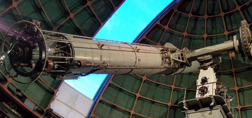
Refracting telescope were the earliest type of optical telescope. Refracting telescopes typically have a lens at the front, then a long tube, then an eyepiece at the rear, where the telescope view comes to focus. The next major step in the evolution of refracting telescopes was the invention of the achromatic lens, a lens with multiple elements that helped solve problems with chromatic aberration and allowed shorter focal lengths. Chromatic aberration is a failure of a lens to focus all colours at the same point (it produces “fringes” of colour along boundaries).
A reflecting telescope uses a single or a combination of curved mirrors that reflect light and form an image. Although reflecting telescopes produce other types of optical aberrations, it is a design that removed chromatic aberration and allowed for very large diameter objectives and shorter focal lengths.
Frederick William Herschel (1738-1822) built his own reflecting telescopes and would discover Uranus, the first planet to be discovered since antiquity. He also pioneered the use of astronomical spectrophotometry, using prisms and temperature measuring equipment to measure the wavelength distribution of stellar spectra. In the course of these investigations, Herschel discovered infrared radiation.
William Parsons, 3rd Earl of Rosse (1800-1867) built in 1845 the “Leviathan of Parsonstown“, the world’s largest (reflecting) telescope, in terms of aperture size (72-inch). He discovered the spiral nature of some nebulae, today known to be spiral galaxies, and the Crab Nebula received its name based on a drawing made by Rosse in the early 1840s.
It was Justus Freiherr von Liebig (1803-1873) proposed a process for silvering that eventually became the basis of modern mirror-making (it was widely adopted only when safety legislation finally prohibited the use of mercury in making mirrors).
Jean Bernard Léon Foucault (1819 -1868) invented the Foucault pendulum, a device demonstrating the effect of Earth’s rotation, and later used the gyroscope as a conceptually simpler experimental proof (see Foucault’s gyroscope experiment). In 1857 Foucault also invented the polariser, and in the succeeding year devised a method to test mirrors of a reflecting telescope to determine its shape. The so-called “Foucault knife-edge test” allows the worker to tell if the mirror was perfectly spherical or has non-spherical deviation in its figure.
The distance to the stars
The first reasonably correct, geometrically grounded measurement of the Earth–Sun distance was by Giovanni Domenico Cassini (1625–1712). Staying in Paris, and with his colleague Jean Richer in Cayenne, French Guiana, the two made simultaneous observations of Mars and, by computing the parallax, determined its distance from Earth. This was the first scientific estimation of the dimensions of the Solar System. Since the relative ratios of various Sun-planet distances were already known from geometry, only a single absolute interplanetary distance was needed to calculate all of the distances. Cassini then derived the Earth–Sun distance at ~140 million km (the modern value is 149.6 million km).
Many early measurements of the Earth-Sun distance were wildly incorrect, and Cassini and Richer arrived at a figure for the solar parallax of 9.5″, equivalent to an Earth–Sun distance of about 22,000 Earth radii. They were also the first astronomers to have access to an accurate and reliable value for the radius of Earth, which had been measured by their colleague Jean Picard in 1669.
The Earth-Sun distance is now an astronomical unit (au) used primarily for measuring distances within the Solar System or around other stars. It is also a fundamental component in the definition of another unit of astronomical length, the parsec. One au is approximately equivalent to 499 light-seconds.
Another colleague of Cassini, Ole Rømer, discovered the finite speed of light in 1676. The speed was so great that it was usually quoted as the time required for light to travel from the Sun to the Earth, or “light time per unit distance”, a convention that is still followed by astronomers today.
Friedrich Wilhelm Bessel (1784-1846) was the first astronomer to determine reliable values for the distance from the Sun to another star (61 Cygni), also by the method of parallax.
Finding our place in the galaxy
Harlow Shapley (1885 -1972) showed that that the Milky Way Galaxy was far larger than previously believed, and that the Sun’s place in the galaxy was in a nondescript location. This discovery supports the Copernican principle, according to which the Earth is not at the centre of the Solar System, the Milky Way galaxy, or the Universe.
Check out the video “Just How Old is the Milky Way Galaxy? | How the Universe Works | Science Channel“.
Before 1908 the only techniques available to astronomers for measuring the distance to a star were based on stellar parallax. Such techniques could only be used for measuring distances out to several hundred light years. It was Henrietta Swan Leavitt (1868-1921) who discovered how to measure vast astronomical distances, which led to a shift in the understanding of the scale and nature of the universe.
Using photographic plates she studied variable stars of the Small and Large Magellanic Clouds, eventually identifying 1,777 variable stars. In 1912 Leavitt looked brightness of a sample of 25 of the Cepheid variables in the Small Magellanic Cloud, and showed that there was a simple relation between the brightness of the Cepheid variables and their periods. All of the Cepheids within the Small Magellanic Cloud were at approximately the same distance, so that their intrinsic brightness could be deduced from their apparent brightness as registered in the photographic plates (but the distance to the Magellanic Clouds was as yet unknown). This soon occurred, allowing her period-luminosity scale to be calibrated. She found that Delta Cepheus was the “standard candle” that had long been sought by astronomers. She also found that a similar five-day cepheid variable in the Small Magellanic cloud was about one ten-thousandth as bright as our five-day Delta Cepheus. Using the inverse-square law, she calculated that the Small Magellanic Cloud was 100 times as far away as Delta Cepheus. This meant she had discovered a way to calculate the distance to another galaxy. The discovery of the period-luminosity relationship for Cepheid variables, is sometimes referred to as Leavitt’s Law.
The expanding Universe
The expanding universe was discovered by separate theoretical and observational work in the 1920s. In 1912–1914, Vesto Slipher discovered that light from remote galaxies was redshifted, a phenomenon later interpreted as galaxies receding from the Earth. In 1922, Alexander Friedmann used the Einstein field equations to provide theoretical evidence that the universe is expanding.
Vesto Melvin Slipher (18751969) was the first to discover that distant galaxies are redshifted, and the first to relate these redshifts to velocity.
A redshift is an increase in the wavelength, or equivalently, a decrease in the frequency, of electromagnetic radiation (such as light). The opposite change, a decrease in wavelength and increase in frequency and energy, is known as a blueshift.
This shift is know as the Doppler Effect (or Doppler shift) is the change in the frequency or, equivalently, the period of a wave in relation to an observer who is moving relative to the source of the wave. It is named after the physicist Christian Doppler, who described the phenomenon in 1842. A common example of Doppler shift is the change of pitch heard when a vehicle approaches and recedes from an observer.
Doppler redshifts is due to the relative motions of radiation sources, gravitational redshift is due to radiation escaping from a gravitational potential, and cosmological redshift is caused by the universe expanding.
In 1912, Slipher measured the first Doppler shift of a “spiral nebula” (the obsolete term for spiral galaxies) and soon discovered that almost all such objects were receding from Earth. By 1917, Slipher had measured the radial velocities of 25 “spiral nebulae,” and found that all but three of those galaxies were moving away from us, at substantial speeds. This was the first data supporting models of an expanding universe, but Slipher did not grasp the full cosmological implications.
In 1922, Alexander Friedmann derived his Friedmann equations from Einstein field equations, showing that the universe might expand at a rate calculable by the equations. In fact, Friedmann describe all three models for the curvature of the universe (positive, zero and negative). It was not until the detection of the cosmic microwave background radiation that the Steady-State model was abandoned in favour of the Big Bang.
The classic solution of the Einstein field equations that describes a homogeneous and isotropic universe is called the Friedmann–Lemaître–Robertson–Walker metric, after Friedmann, Georges Lemaître, Howard P. Robertson and Arthur Geoffrey Walker, who worked on the problem in the 1920s and 30s independently of Friedmann.
Edwin Hubble observed Cepheid variable stars in “spiral nebulae”, which enabled him to calculate the distances to these objects. Surprisingly, these objects were discovered to be at distances which placed them well outside the Milky Way. They continued to be called nebulae, and it was only gradually that the term galaxies replaced it. Combining his measurements of galaxy distances with Vesto Slipher and Milton Humason‘s measurements of the redshifts associated with the galaxies, Hubble discovered a rough proportionality between redshift of an object and its distance. The Hubble–Lemaître law, is the observation that galaxies are moving away from Earth at speeds proportional to their distance. In other words, the farther a galaxy is from the Earth, the faster it moves away.
At the time this overturned the notion of a Static Universe. This meant that the universe was evolving, and that it must have had a definite beginning.
It’s worth noting that the “Hubble constant“, is a misnomer since it is constant in space only at a fixed time. It varies with time in nearly all cosmological models, and all observations of far distant objects are also observations into the distant past, when the “constant” had a different value.
It’s worth checking out some videos on these topics:-
The Universe’s Expansion No Longer Makes Sense
Why Does Galaxy Redshift Mean the Universe is Expanding?
The Man Who Corrected Einstein (Alexander Friedmann)
Discovering Our Universe – Celebrating the Centennial of Edwin Hubble’s Remarkable Journey
New big telescopes
Telescope mounts can be fixed in one position, such as zenith telescopes (just point straight up at or near the zenith). Or they can be fixed-altitude mounts with optics fixed at an altitude angle while rotating horizontally (in azimuth). Or they can be transit mounts which are single axis mounts fixed in azimuth while rotating in altitude, usually oriented on a north-south axis. Or they can be altazimuth mount (alt-az) that moved in altitude (up and down), or azimuth (side to side), as separate motions. There is an altitude-altitude mounts (alt-alt), that has the advantage of not having a blind spot near the zenith. And there is the equatorial mount that has north-south “polar axis” tilted to be parallel to Earth’s polar axis that allows the telescope to swing in an east-west arc, with a second axis perpendicular to that to allow the telescope to swing in a north-south arc.
A transit instrument is a small telescope with an extremely precisely graduated mount used for the precise observation of star positions. They can be Meridian instruments are for observation of star transits in the exact direction of South or North, e.g. meridian circles (for timing of the passage of stars across the local meridian), mural quadrants (an angle measuring instrument mounted on or built into a wall), etc. Or they can be a zenith telescope, a very simple design that just points straight up at or near the zenith, and is used for precision measurement of star positions.
An altazimuth mount (alt-azimuth) is a simple two-axis mount for supporting and rotating an instrument about two perpendicular axes, one vertical and the other horizontal. A gun turret is essentially an alt-azimuth mount for a gun, and a standard camera tripod is an alt-azimuth mount as well. They can look at any point in the sky but can’t follow astronomical objects in the night sky as the Earth spins on its axis (they need a microprocessor based two-axis drive systems, to track equatorial motion).
An equatorial mount is a mount for instruments that compensates for Earth’s rotation by having one rotational axis, called polar axis, parallel to the Earth’s axis of rotation. The advantage of an equatorial mount it can stay fixed on any celestial object with diurnal motion by driving one axis at a constant speed.
Check out the videos:-
Understanding Telescope Mounts
New big mirrors
How to make a telescope mirror
How to grind a mirror for a telescope
Making Large Telescope Mirrors
Go Inside a Telescope Mirror Factory | To a Billionth of a Meter
Here are some videos on big/new telescopes:-
The European Southern Observatory (ESO) has a YouTube Channel. It has numerous videos on both the Very Large Telescope and the Extremely Large Telescope.
Planets and Stars with Keck Observatory and the James Webb Telescope
GIANT Magellan Telescope is Made of 7 HUGE Mirrors & Won’t Produce Diffraction Spikes
Effects of the atmosphere
The Earth’s atmosphere is not totally transparent and is in fact 100% opaque to many wavelengths. The wavelength ranges to which it is transparent are called atmospheric windows. These windows, especially the optical and infrared, affect the distribution of energy flows and temperatures within Earth’s energy balance. The windows are themselves dependent upon clouds, water vapour, trace greenhouse gases, and other components of the atmosphere. The optical, infrared and radio windows comprise the three main atmospheric windows.
The optical window is the portion of the optical spectrum that is not blocked by the Earth‘s atmosphere. The window runs from around 300 nanometers (ultraviolet-B) up into the range the human eye can detect, roughly 400–700 nm and continues up to approximately 2 μm. Sunlight mostly reaches the ground through the optical atmospheric window, and the Sun is particularly active in most of this range (44% of the radiation emitted by the Sun falls within the visible spectrum and 49% falls within the infrared spectrum).
The infrared atmospheric window is an atmospheric window in the infrared spectrum where there is relatively little absorption of terrestrial thermal radiation by atmospheric gases.
The radio window is the region of the radio spectrum that penetrate the Earth’s atmosphere.
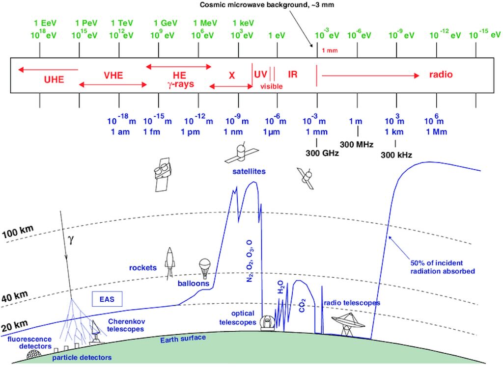
The above diagram summarises the transparency of the Earth’s atmosphere to electromagnetic radiation over the full spectrum, from γ-rays to radio waves. The horizontal axis represents wavelength (and equivalent photon energy), while the vertical transmission curve indicates which spectral regions can reach the Earth’s surface.
At very short wavelengths (γ-rays and X-rays), the atmosphere is essentially opaque due to strong absorption and ionisation processes in the upper atmosphere, so observations in these bands require satellite-based instruments. In the ultraviolet, absorption by molecular oxygen and ozone further blocks most radiation below ~300 nm.
Two major atmospheric transmission windows are evident. The first is the visible/near-infrared optical window, where atmospheric absorption is relatively low, enabling ground-based optical telescopes. The second is the broad radio window at long wavelengths (metre to centimetre scales), where atmospheric attenuation is negligible and radio telescopes operate effectively from the ground.
Between these windows, particularly in the infrared and submillimetre/terahertz region, transmission is strongly reduced by molecular absorption bands of water vapour and carbon dioxide, motivating high-altitude observatories, balloon experiments, rockets, or space telescopes depending on wavelength.
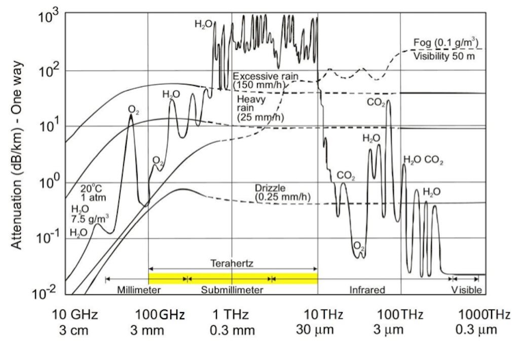
Now the above more detailed diagram shows the attenuation of electromagnetic radiation by the Earth’s atmosphere as a function of frequency and equivalently, wavelength, with attenuation (vertical axis), expressed in dB per kilometre (dB/km) for a one-way path through the atmosphere.
It therefore quantifies how transparent or opaque the atmosphere is to radiation across the electromagnetic spectrum, from millimetre and submillimetre waves. through to infrared and visible light. The figure is essentially a map of the atmospheric transmission windows that determine where ground-based optical telescopes can operate.
The vertical axis gives the loss of signal intensity per kilometre of atmospheric path, in logarithmic units, where 1 dB/km means moderate absorption/scattering, 10 dB/km means strong attenuation, and 100–1000 dB/km means the radiation is essentially blocked over short distances. The scale is logarithmic, and span from very transparent (10-2 dB/km) to extremely opaque (103 dB/km). The label “One way” means the attenuation applies to a single pass through the atmosphere, not a round-trip (important in radar, but astronomy is one-way).
The bottom axis covers centimetre radio to visible optical.
The sharp peaks and troughs in the curves are caused by dominant molecular absorption lines in the atmosphere, H₂O (water vapour), O₂ (oxygen) and CO₂ (carbon dioxide). These gases absorb radiation at specific frequencies due to quantised molecular transitions, i.e. rotational transitions (microwave/sub-mm) and vibrational transitions (infrared).
On the left we have the atmospheric radio window from roughly 10 GHz to tens of GHz, where attenuation is extremely low 10-2 to 10-1 dB/km. This is the radio window, which allows ground-based radio astronomy.
The diagram shows a strong peak labelled O₂ near ~60 GHz. This corresponds to oxygen rotational absorption lines, which produce a major opacity band.
Beyond ~100 GHz (3 mm), attenuation increases due mainly to water vapour (H₂O). The diagram shows multiple sharp H₂O absorption lines. This is why mm/sub-mm telescopes require high, dry sites.
Im the Terahertz band (0.1–10 THz) wavelengths from ~3 mm down to ~30 µm attenuation rises dramatically 10–1000 dB/km). This is because water vapour has an extremely dense absorption structure in this range. Thus ground-based THz astronomy is severely limited. Most THz astronomy requires space telescopes. The yellow-highlighted bar marks this “Terahertz gap”.
In the infrared, attenuation is dominated by H₂O and CO₂ vibrational bands. The diagram shows a major CO₂ absorption feature around ~30 THz (~10 µm) and strong H₂O bands throughout. However, there are infrared atmospheric windows, especially near 1–2 µm (near-IR), 3–5 µm (mid-IR partial window) and 8–13 µm (thermal IR window). This is why infrared observatories exist on high mountains.
At the far right, labelled “Visible”, attenuation drops again to very low values. The atmosphere is highly transparent in the optical band, and ground-based optical astronomy is possible. The visible window exists because major atmospheric gases do not strongly absorb visible photons, and scattering is present but not fully opaque.
The diagram also includes dashed curves showing attenuation from hydrometeors. Drizzle (0.25 mm/h) adds modest attenuation, mostly at higher frequencies. Heavy rain (25 mm/h) is strongly attenuating in the microwave and mm bands. Excessive rain (150 mm/h) absorbs and scatters. Fog (0.1 g/m³, visibility 50 m) produces very large attenuation in optical/IR because droplets scatter strongly. These curves show that transparency depends not only on gases but also on liquid water content.
Atmospheric blurring
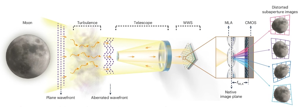
Atmospheric turbulence can be regarded as spatially variant aberrations that manifest themselves as phase modulations of the pupil plane. Conventional imaging devices are limited to detecting the intensity information of three-dimensional (3D) scenes projected onto a two-dimensional (2D) sensor, and are unable to capture phase disturbances. To overcome this limitation, a wide-field wavefront sensor (WWS) uses a micro-lens array (MLA) at the image plane with a complementary metal–oxide–semiconductor (CMOS) sensor placed at the back focal plane of the MLA to detect the spatial variance of the coherence in a parallel way. The above graphics is taken from “Direct observation of atmospheric turbulence with a video-rate wide-field wavefront sensor“.
For more background, check out atmospheric turbulence.
Atmospheric turbulence defines the effective angular resolution of grand-based optical telescopes, and is driven by winds mixing cool and warm air, creating high- and low-density pockets.
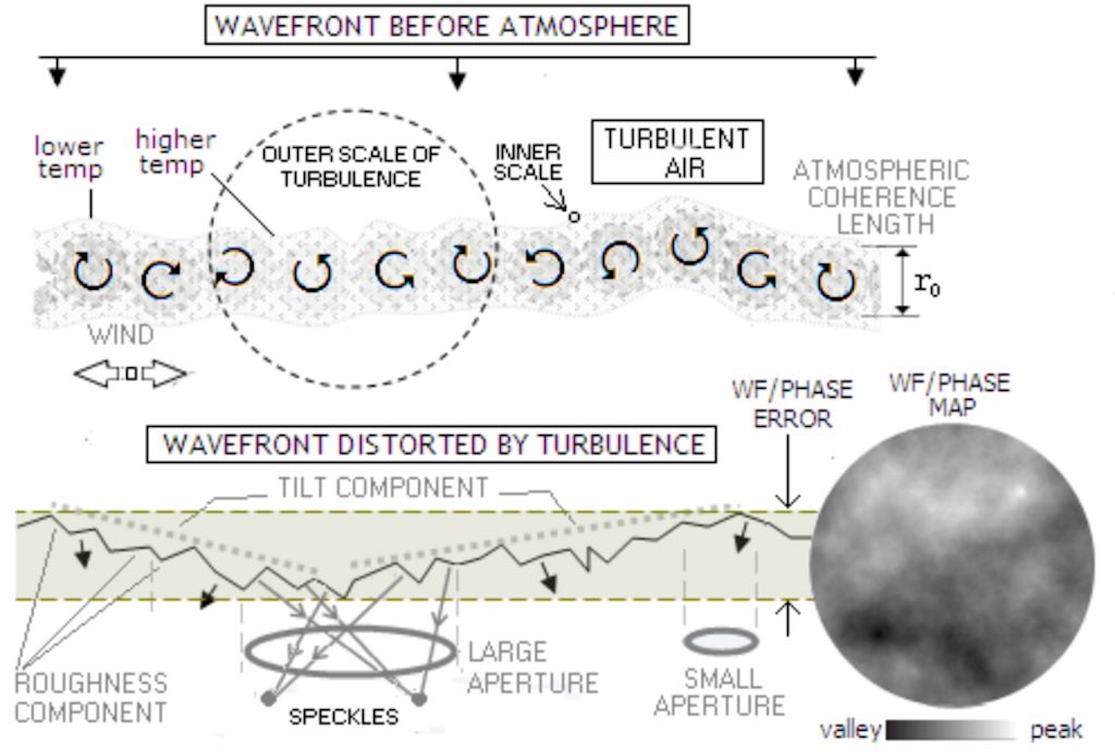
Astronomical seeing is the degradation of the image of an astronomical object due to turbulence in the atmosphere of Earth that may become visible as blurring, twinkling or variable distortion. The origin of this effect is rapidly changing variations of the optical refractive index along the light path from the object to the detector. Seeing is a major limitation to the angular resolution in astronomical observations with telescopes that would otherwise be limited through diffraction by the size of the telescope aperture. Today, many large scientific ground-based optical telescopes include adaptive optics to overcome seeing.
Airglow
The above discussed transmission (opacity vs transparency). However, the Earth’s atmosphere also produces natural emission known as airglow (notably O and OH bands), which contributes to the optical and near-infrared night-sky background and limits the sensitivity of ground-based observations.
Airglow originates mainly in atmospheric layers around ~80–100 km (mesosphere/lower thermosphere), and up to ~300 km (ionospheric regions). So it is well above weather and tropospheric absorption.
Airglow is the natural emission of light by the Earth’s upper atmosphere, caused by atoms and molecules that have been excited by solar ultraviolet radiation during the day, chemical reactions in the mesosphere and thermosphere, and the recombination of ions and electrons at night. So it is an emission phenomenon, not absorption. It adds a natural background light that limits sensitivity, and as such it affects astronomy through sky brightness, not through blocking radiation.
The strongest contributors to natural night-sky brightness and 557.7 nm (green oxygen line), and 630.0 nm (red oxygen line).
There is also a near-infrared airglow, the Meinel bands (0.8–2.0 µm), that make the near-infrared sky much brighter from the ground than from space.
Adaptive optics
Recording images
The supermassive black hole in the centre of the Milky Way
Sky surveys
Robotic telescopes and the discovery of extrasolar planets
During
Two future optical telescopes
During